
Impedance Control of a Redundant Parallel Manipulator
Juan de Dios Flores Mendez
1
, Henrik Schiøler
1
, Ole Madsen
2
and Shaoping Bai
2
1
Department of Electronic Systems, Aalborg University, Frederik Bajers Vej 7C, 9220, Aalborg East, Denmark
2
Department of Mechanical and Manufacturing Engineering, Aalborg University,
Fibigerstraede 16, 9220, Aalborg East, Denmark
Keywords:
Robotics, Redundant Parallel Manipulators, Control, Optimization, Compliant Motion, Impedance Control.
Abstract:
This paper presents the design of Impedance Control to a redundantly actuated Parallel Kinematic Manipulator.
The proposed control is based on treating each limb as a single system and their connection through the internal
interaction forces. The controller introduces a stiffness and damping matrices that decouples the dynamic
behaviour of the robot. Control allocation of torques is applied through an optimization that promotes even
distribution of torques over actuators. Simulations showed a good compliance behaviour in low frequencies.
1 INTRODUCTION
Parallel Kinematic Manipulators (PKMs) have been
mainly used in pick and place operations or posi-
tioning systems in manufacturing due to their high
speed, high accelerations and low inertia (Patel and
George, 2012), with applications such as assembly
(McCallion and Pham, 1979), positioning (Ming and
Higuchi, 1994), motion simulators (Salcudean et al.,
1994), pick and place (Powell, 1982), and material
processing operations such as drilling (Company and
Pierrot, 2002).
The inherent stiffness of the PKMs and higher
speed (Taghirad, 2013) than the serial kinematic ma-
nipulators make them ideal for performing different
tasks in the manufacturing sectors such as assembly
and material processing (Schutz and Wahl, 2011).
The tasks of assembly, material processing as
polishing or de-burring and material handling are
tasks that require compliant motions (Bruyninckx and
Schutter, 1996) i.e. the robot required to adapt the
torques and forces when in contact with environmen-
tal objects.
An approach to compliant motion is the so called
Impedance Control (Hogan, 1985). Impedance Con-
trol is classified as an indirect force control because is
designed to avoid the necessity to measure the force in
the mobile platform. The aim of Impedance Control
is to impose a desired apparent mechanical stiffness
and damping in the Cartesian space of the robot. In
a robotic system that can perform 3 translations by 3
actuators, it becomes a straight forward task because
there is a one to one mapping from the Cartesian space
to the actuator space. In a robotic system with actua-
tor redundancy it is not a trivial task.
PKMs with redundant actuation are those that
have more actuators than degrees of freedom. The
control of redundant PKMs requires the solution of
inverse dynamics which is not straight forward and
techniques as the Moore-Penrose pseudo inverse ma-
trix (Briot et al., 2013) or the null space of the forces
is used (Kock and Schumacher, 2011) to solve this
problem. There are advantages of redundant actuated
robots such as improvement of Cartesian stiffness
within the worspace, homogeneous symmetric force
output and a need for optimization due to the fact
that the dynamic equations are indeterminate (Cheng
et al., 2001).
Recently, the BlueWorkforce company (Hjørnet,
2016) developed a new industrial redundant PKM
(The Ragnar Robot) with an optimized extended
workspace and relatively low price. By optimizing
the mechanical design and force transmission it was
possible to change materials and reduce costs.
The motivation behind the work presented in this
paper is to introduce compliant motion control in re-
dundantly actuated PKMs such as the Ragnar robot
for optimization to perform different compliant mo-
tion tasks in a manufacturing environment.
In this paper, we proposed an impedance con-
troller for a redundant parallel manipulator by setting
a desired stiffness and damping for each coordinate
axis in the cartesian space. The proposed method
considers every limb as a separate system. Limb dy-
104
Mendez, J., Schiøler, H., Madsen, O. and Bai, S.
Impedance Control of a Redundant Parallel Manipulator.
DOI: 10.5220/0006433301040111
In Proceedings of the 14th International Conference on Informatics in Control, Automation and Robotics (ICINCO 2017) - Volume 1, pages 104-111
ISBN: 978-989-758-263-9
Copyright © 2017 by SCITEPRESS – Science and Technology Publications, Lda. All r ights reserved
namic equations are coupled through internal inter-
action forces in the attachment points of the mobile
platform. Impedance control is designed as a decou-
pled stiffness and damping for each direction of the
coordinate axes.
The paper is organized as follows: In Section 2
the parallel kinematic manipulator is described. Sec-
tion 3 briefly describes the kinematics of the manip-
ulator. The dynamic model on which the impedance
controller is based is described in Section 4. The tra-
jectory generation and inverse dynamics of the redun-
dant parallel robot is discussed in Section 5. The set-
ting for the impedance controller and optimization is
described in Section 6. In Section 7 simulations and
results are presented for the proposed method. Sec-
tion 8 presents a brief conclusion.
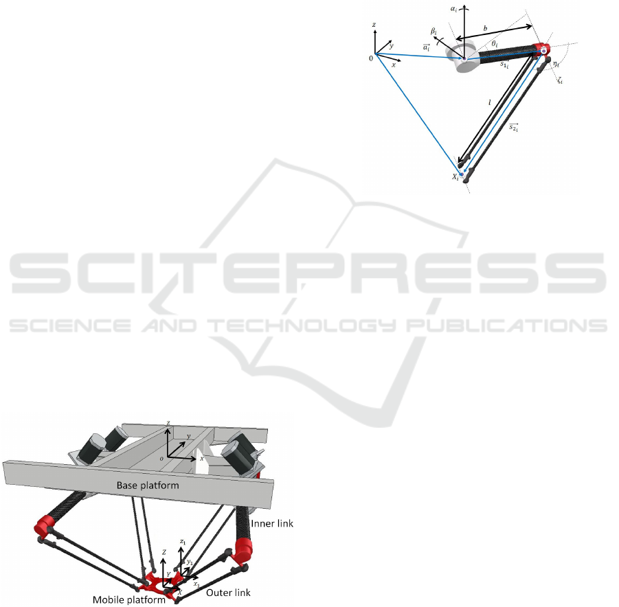
2 SYSTEM DESCRIPTION
The Ragnar parallel robot is a four limbs redundant
parallel robot designed for 3D mobility of its mo-
bile platform, while mechanically fixed in a constant
orientation. Each limb comprises an actuated inner
link attached to the base platform and an outer link
attached to the mobile platform. The global coordi-
nate system is located in the center of the base plat-
form, the mobile coordinate system is located to the
center of the mobile platform (center piece) and four
auxiliary local coordinate systems are located to the
connection between the mobile platform and each of
the outer links. The figure shows the location of the
global coordinate system, the mobile platform coordi-
nate system and the first auxiliary coordinate system
at the attachment point.
Figure 1: Ragnar robot with location of the coordinate sys-
tems.
3 KINEMATIC ANALYSIS
The kinematic constraint equations are given by a set
of generalized coordinates q
i
that can describe the po-
sition of one leg. The set of generalized coordinates
chosen is composed by the active and passive joint an-
gles of one limb, i.e. q
i
=
θ
i
ζ
i
η
i
T
. The active
joint angle θ
i
, passive joint angles ζ
i
,η
i
and geometric
parameters are shown in the figure below.
Figure 2: Generalized coordinates.
Let x
i
denote the position of the i-th attachment
point of the mobile platform and the limb. Then, the
position vector of x
i
in global coordinates is
~a
i
+
~
s
1
i
+
~
s
2
i
= x
i
(1)
Rewriting Eq. (1) in local vectors
~a
i
+ R
1
i
~
b
i
+ R
1
i
R
2
i
~
l
i
= x
i
(2)
Where R
1
i
denotes the rotation of the actuated joint
and R
2
i
the rotation of the passive joint
R
1
i
= R
α
i
z
R
β
i
y
R
θ
i
z
(3)
R
2
i
= R
ζ
i
z
R
η
i
y
(4)
where α
1,3
= −α
2,4
= π/12, −β
1,4
= β
2,3
= π/4 and
the local vectors
~
b
i
and
~
l
i
defined as
~
b
i
= b
i
~
i
~
l
i
= l
i
~
i (5)
where
~
i stands as the unit vector in the x direction of
the i-th coordinate system. The solution to the in-
verse geometric problem is solved using a the well
known spherical-spherical constraint (Garcia de Jalon
and Bayo, 1994) and described in (Wu et al., 2016).
3.1 Jacobian Analysis
Differentiating Eq. (2) with respect to time we get the
Jacobian for each separate limb.
˙x
i
= J
i
˙q
i
(6)
Impedance Control of a Redundant Parallel Manipulator
105

with
J
i
=
j1
i
j2
i
j3
i
(7)
where
j1
i
= R
1
i
~
k ×
~
b
i
+ R
2
i
~
l
i
(8)
j2
i
= R
1
i
R
ζ
i
z
~
k × R
η
i
y
~
l
i
(9)
j3
i
= R
1
i
R
2
i
~
j ×
~
l
i
(10)
This allows to obtain four jacobians for a singular po-
sition that allow the calculation of all the velocities of
the joints of the robot. Let x denote the position of the
mobile platform, then its position can be described by
x = x
i
+ d
i
(11)
where d
i
is a constant vector from the i-th attachment
point to the mobile platform. Deriving Eq. (11) with
respect to time yields
˙x = ˙x
i
(12)
which implies
˙x = J
i
˙q
i
(13)
4 DYNAMIC MODELING
The dynamic model is derived first in each limb and
then are combined with the dynamic formulation of
the mobile platform.
4.1 Dynamic Model of the Limb
The dynamics is computed using the variational
method of the Lagrange equations.
The Lagrange equation is defined as
d
dt
∂L
i
∂ ˙q
i
−
∂L
i
∂q
i
= Q
ext
i
(14)
And the Lagrangian
L
i
≡ T
i
−V
i
(15)
where Q
ext
i
= τ
i
− J
T
i
f
i
are the external forces, τ
i
=
T
i
0 0
T
is the actuator torque and f
i
is an interac-
tion force in the attachment point. The center of mass
of the inner link and the outer link are considered to
be at the center of each link. Furthermore, the kinetic
energy associated to the rotation of the outer link is
deprecated for simplification. Figure 3 shows the ex-
ternal forces acting in the limb and Figure 4 shows the
location of the center of mass of the limbs.
The kinetic energy T
i
of the i-th limb is calculated
as
T
i
=
1
2
I
b
˙
θ
2
i
+
1
8
m
b
˙
~
s
1
i
2
+
1
2
m
l
˙
~
s
1
i
+
1
2
˙
~
s
2
i
2
(16)
Figure 3: Torque, interaction force and gravity on the i-th
limb.
Figure 4: Center of mass of the links.
and the potential energy V
i
of the i-th limb as
V
i
= m
b
1
2
~
s
1
i
T
g + m
l
~
s
1
i
+
1
2
~
s
2
i
T
g (17)
where I
b
and m
b
is the inertia and mass of the inner
link and m
l
is the mass of the outer link.
Deriving the equations gives as a result an dy-
namic equation for the i-th limb in the form
M
i
(q
i
) ¨q
i
+C( ˙q
i
,q
i
) + G(q
i
) = τ
i
− J
T
i
f
i
(18)
4.2 Dynamic Model of the Mobile
Platform
The rotation of the mobile platform is mechanically
fixed, thus the dynamic equation is derived as
M
p
¨x + G
p
= f
e
+
4
∑
i=1
f
i
(19)
where M
p
= m
p
I
3
denotes the mass of the mobile plat-
form times the identity matrix, f
i
the effect of the in-
teraction forces in the i-th attachment point G
p
is the
gravity vector of the mobile platform and f
e
is the in-
terface force between the mobile platform and the en-
vironment.
The full dynamic model of the robot is derived
combining Eq. (18) and Eq. (19)
ICINCO 2017 - 14th International Conference on Informatics in Control, Automation and Robotics
106

Figure 5: Forces acting on the mobile platform.
5 REFERENCE TRAJECTORY
The compliant motion of the robot is achieved when
the robot deviates from its trajectory in response to
the forces resulting from the robot interacting with an
external object.
Given a reference trajectory as the set of posi-
tions, velocities and accelerations of the mobile plat-
form i.e. {x
r
, ˙x
r
, ¨x
r
}, we can compute the set of po-
sitions, velocities and accelerations of the joints i.e.
{q
r
i
, ˙q
r
i
, ¨q
r
i
}.
In a non-redundant robot, the torques of the mo-
tors can be determined through Eq. (18) and Eq. (19).
In a redundantly actuated robot the torques for the
motors cannot be determined directly through the dy-
namic equations. The inverse dynamics of the robot
yields to three equations for translational motion and
four torque inputs to be determined.
5.1 Reference Trajectory with
Optimized Torques
The trajectory given in a set of the mobile plat-
form and joints positions, velocities and accelerations
{x
r
, ˙x
r
, ¨x
r
,q
r
i
, ˙q
r
i
, ¨q
r
i
}. The aim is to determine the
value references of torques for the given trajectory.
The torque equation for a reference trajectory of
the i-th limb becomes
τ
r
i
= M
i
¨q
r
i
+C( ˙q
r
i
,q
r
i
) + G(q
r
i
) + J
T
r
i
f
r
i
∀ = 1..4
(20)
and all the torque equations are combined with the
translational motion equation of the mobile platform
in absence of external forces, i.e.
M
p
¨x
r
+ G
p
=
4
∑
i=1
f
i
r
(21)
Eqs. (21) and (20), given the reference trajectory
form a set of 15 equations and 16 variables, thus the
solution for the inverse dynamics can have infinite so-
lutions. The problem can be set as an optimization
problem where the objective function can be selected,
along with constraints, to support additional design
specifications as well as to remove the ambiguity of
the solution for actuator torques. In this paper the ob-
jective function is chosen to promote even distribution
of the torques over actuators. We chose the objective
function as follows
f
ob j
( f
i
) =
4
∑
i=1
T
2
i
(22)
The optimization setting for finding the reference
torques and forces, by combining Eq. (22), Eqs. (20)
and Eq. (21) i.e.
min f
ob j
( f
i
) st
M
p
¨x
r
+ G
p
−
4
∑
i=1
f
i
r
= 0
τ
r
i
= M
i
¨q
r
i
+C( ˙q
r
i
,q
r
i
) + G(q
r
i
) + J
T
r
i
f
i
∀i = 1..4
τ
r
i
= [T
r
i
0 0]
T
∀i = 1..4
τ
≤ τ
r
i
≤
¯
τ ∀i = 1..4
(23)
where τ and
¯
τ stand for the minimum and maximum
torques of the motor. Defining
h
a
= [1 0 0] (24)
h
b
=
0 1 0
0 0 1
(25)
we may reformulate Eq. (23) as
min
f
1
,.., f
4
4
∑
i=1
(h
a
τ
r
i
)
2
st
M
p
¨x
r
+ G
p
−
4
∑
i=1
f
i
r
= 0
h
b
τ
r
i
= 0 ∀i = 1..4
τ − h
a
τ
r
i
≤ 0 ∀i = 1..4
h
a
τ
r
i
−
¯
τ ≤ 0 ∀i = 1..4 (26)
upon which reference torques T
r
i
and internal interac-
tion forces f
r
i
are found.
6 IMPEDANCE CONTROL
Impedance control specifies a stiffness (k
p
) and damp-
ing (k
v
) to the mobile platform.
Taking Eq. (19) and renaming the sum of the in-
ternal interaction forces as a controlled forces f
c
it can
be re written as
M
p
¨x + G
p
= f
e
+ f
c
+ f
r
(27)
Impedance Control of a Redundant Parallel Manipulator
107

by subtracting
M
p
¨x
r
= f
r
− G
p
(28)
we obtain
M
p
δ ¨x = f
e
+ f
c
(29)
with
δx = x − x
r
(30)
and set the desired damping and stiffness in the mo-
bile platform, named the damping (K
p
) and stiffness
(K
v
) matrices with a gravity compensator
f
c
= − (K
p
δx + P
v
δ ˙x) (31)
Inserting Eq. (31) into Eq. (27) we get
M
p
δ ¨x = f
e
− (K
p
δx + K
v
δ ˙x) (32)
As a result, we obtain a relationship suitable for the
design of an impedance controller, i.e.
M
p
δ ¨x + K
v
δ ˙x + K
p
δx = f
e
(33)
The damping and stiffness matrices are usually
chosen to be diagonal in order to decouple the dy-
namic effects in each direction of the Cartesian space.
6.1 Inverse Kinematics Approximation
Assuming that the robot position is sufficiently close
to the reference trajectory the inverse kinematics ap-
proximate linearly as
δx
i
= x
i
− x
r
i
≈ J
i
(q
r
i
)(q
i
− q
r
i
) = J
i
(q
r
i
)δq
i
(34)
or
δq
i
≈ J
−1
i
(q
r
i
)δx
i
(35)
Defining
J (t) = J
−1
i
(q
r
i
(t))
we obtain
δ ˙q
i
≈
˙
J δx
i
+ J δ ˙x
i
(36)
and
δ ¨q
i
≈
¨
J δx
i
+
˙
J δ ˙x
i
+
˙
J δ ˙x
i
+ J δ ¨x
i
(37)
≈
¨
J δx
i
+ 2
˙
J δ ˙x
i
+ J δ ¨x
i
(38)
We shall convert the limb i torque equation (18) into
dynamics for x
i
by a simplified linear approximation,
i.e.
δτ
i
= τ
i
− τ
r
i
≈ M(q
r
i
)δ ¨q
r
i
+ G(q
r
i
)
q
δq
i
+ J(q
r
i
)δ f
i
(39)
Finally, inserting Eq. (35), Eq. (36) and Eq. (38) into
Eq. (39) we get an approximation of the limb i torque
equation in terms of δx
i
6.2 Control Allocation
Similarly to Section 5 the problem is set up in an
optimization. The torques are allocated through
an optimization that promotes even distribution of
torques, thus reducing the sudden change of manip-
ulator torques. The optimization is set up using the
objective function previously defined in Eq. (22), i.e.
min f
ob j
( f
i
) st
K
p
δx + K
v
δ ˙x +
4
∑
i=1
f
i
− G
p
= 0
δτ
i
= M(q
r
i
)δ ¨q
r
i
+ G(q
r
i
)
q
δq
i
+ J(q
r
i
)δ f
i
∀i = 1..4
τ
i
= [T
i
0 0]
T
∀i = 1..4
τ ≤ τ
i
≤
¯
τ ∀i = 1..4
(40)
and with further calculations
min
4
∑
i=1
(h
a
(δτ
i
+ τ
r
))
2
st
K
p
δx + K
v
δ ˙x +
4
∑
i=1
f
i
− G
p
= 0
h
b
(δτ
i
+ τ
r
) = 0 ∀i = 1..4
τ − h
a
(δτ
i
+ τ
r
) ≤ 0 ∀i = 1..4
h
a
(δτ
i
+ τ
r
) −
¯
τ ≤ 0 ∀i = 1..4 (41)
where
T
i
= h
a
(δτ
i
+ τ
r
) (42)
δτ
i
= M(q
r
i
)δ ¨q
r
i
+ G(q
r
i
)
q
δq
i
+ J(q
r
i
)δ f
i
(43)
7 SIMULATION AND RESULTS
7.1 Simulation Setup
The masses and geometric parameters are taken from
a CAD model of the robot. The controller and the dy-
namic model of the robot are simulated numerically.
Table 1 shows the geometric and physical parameters
of the robot.
7.1.1 Static Reference
The proposed method is evaluated, as the beginning
of our investigation, in a static position ( ¨x
r
= ˙x
r
= 0)
i.e. the reference trajectory. The reference position is
the initial position of the robot, which is selected to be
x = [0 0 −0.4]
T
. For the case of a non-static reference
trajectory we can also apply the same procedure to
find the reference forces and torques.
ICINCO 2017 - 14th International Conference on Informatics in Control, Automation and Robotics
108
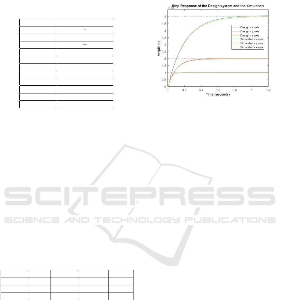
Table 1: Geometrical and physical parameters of the Ragnar
Robot.
Parameter Value
γ
π
6
a
i
[±0.28,∓0.114][m]
α
π
12
b 0.3[m]
l 0.55[m]
r 0.1[m]
m
p
0.25[kg]
m
b
0.3[kg]
I
b
0.0013[kg · m
2
]
m
l
0.12[kg]
max. torque 10[Nm]
7.2 The Stiffness and the Damping
Matrices
The stiffness and Damping matrices are selected to be
diagonal in order to decouple the stiffness and damp-
ing responses in Cartesian space. We selected the
following stiffness and damping matrices, for which
the poles of each transfer function are different. We
selected different stiffness gains for evaluation pur-
poses and selected different cut-off ( f r) frequencies
for each axis to compute the damping.
K
p
=
K
px
0 0
0 K
py
0
0 0 K
pz
(44)
K
v
=
K
vx
0 0
0 K
vy
0
0 0 K
vz
(45)
Table 2: Stiffness and Damping design parameters.
Stifness [N/m] f r [s
−1
] Damping [Ns/m]
K
px
1000 30 K
vx
40.83
K
py
500 10 K
vy
52.5
K
pz
200 5 K
vz
41.25
7.3 Step Response
A step response is applied to the system in each of the
cartesian axis and is compared to the desired step re-
sponse. The step input applied at t = 0 is f
e
= [1 1 1]
T
The results are shown below.
It is observed that the step response of the simula-
tion and the desired response is as expected with the
largest error in the z-axis.
From the data of the simulation it was calculated
the following constant of time for each of the step re-
Figure 6: Step response of the simulation and the desired
response.
sponses as
τ
t
x
= 0.0355 (46)
ω
x
= 1/τ
t
x
= 28.16 (47)
τ
t
y
= 0.096 (48)
ω
y
= 1/τ
t
y
= 10.41 (49)
τ
t
z
= 0.207 (50)
ω
z
= 1/τ
t
z
= 4.83 (51)
where the poles resulting from the selection of stiff-
ness and damping in the design phase are
p
x1
= −30 p
x2
= −133.33 (52)
p
y1
= −10 p
y2
= −200 (53)
p
z1
= −5 p
z2
= −160 (54)
We observed that the error of the measured cut off
frequencies from the simulation, that correspond to
the dominant poles, are very close to the design re-
quirement. The measured absolute errors are
e
x
= 1.84 (55)
e
y
= 0.41 (56)
e
z
= 0.17 (57)
where the maximum error is measured in the x-axis
possibly due to the approximations previously out-
lined.
7.4 Response to Harmonic Forces
In the last section a step response was applied to eval-
uate the desired response of the system against the
simulation but is only valid for very low frequencies.
The designed system is simulated for the case of ex-
ternal harmonic forces acting in the mobile platform.
The harmonic forces are in the form
f
he
= A sin(2π · ω ·t) (58)
Impedance Control of a Redundant Parallel Manipulator
109
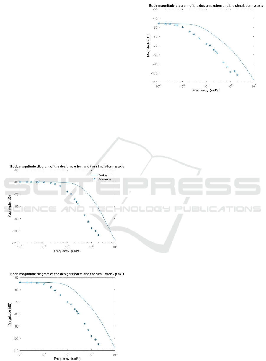
An amplitude of A = 1 is selected for the harmonic
forces and frequency is varied to obtain a sketch of the
Bode plot of the simulated system with controller.
The external harmonic force is simulated as
f
e
(t) = [ f
he
f
he
f
he
]
T
7.4.1 Bode Plot Comparison
Figures 7, 8 and 9 show the results from the simula-
tion of the system when harmonic forces are applied
to the mobile platform. The harmonic forces were ap-
plied in the direction of the three axis of the global co-
ordinate system. Then, the gain was computed from
the simulation. Different frequencies were applied to
the system to test the controller and obtain the Bode
plot of the system with the controller.
Comparing the response to harmonic forces in dif-
ferent frequencies we observe that the cut-off fre-
quency is almost half decade behind the designed cut
off frequency. This can be caused due to the small
difference of the mass of the mobile platform and the
limbs, which does not allow for many simplifications
Figure 7: Bode plot of the simulation and the desired re-
sponse in x-axis.
Figure 8: Bode plot of the simulation and the desired re-
sponse in y-axis.
Figure 9: Bode plot of the simulation and the desired re-
sponse in z-axis.
but could be mitigated when the mass of the mobile
platform is increased when there is a tool attached to
it.
8 CONCLUSIONS
In this paper was presented the case for impedance
control for a redundant parallel robot. The impedance
control is based on linearisation of the robot dynam-
ics around a reference trajectory. We showed that
the controller works in a region close to the refer-
ence trajectory and its response to harmonic forces
differs to the design but the step response is as de-
signed with small error but it increases when the stiff-
ness or damping is reduced. The simulation showed
that the system has a time constant similar to the de-
sign requirement on each axis.
Since the Ragnar robot is a redundantly actuated
parallel robot, its inverse dynamics is indeterminate
and an optimization is applied to obtain torques. Fu-
ture work includes the implementation of the de-
signed controller on the Ragnar robot as well as ap-
plying the compliance approach presented in this pa-
per in an iterative learning framework for improved
performance in eg. assembly.
REFERENCES
Briot, S., Gautier, M., and Krut, S. (2013). Dynamic pa-
rameter identification of actuation redundant parallel
robots: Application to the dualv. In AIM: Advanced
Intelligent Mechatronics, Jul 2013, Wollongong, Aus-
tralia. IEEE/ASME, pages pp.637–643.
Bruyninckx, H. and Schutter, J. D. (1996). Specification of
force-controlled actions in the ldquo;task frame for-
malism rdquo;-a synthesis. IEEE Transactions on
Robotics and Automation, 12(4):581–589.
ICINCO 2017 - 14th International Conference on Informatics in Control, Automation and Robotics
110

Cheng, H., Liu, G. F., Yiu, Y. K., Xiong, Z. H., and Li,
Z. X. (2001). Advantages and dynamics of paral-
lel manipulators with redundant actuation. In Pro-
ceedings 2001 IEEE/RSJ International Conference on
Intelligent Robots and Systems. Expanding the Soci-
etal Role of Robotics in the the Next Millennium (Cat.
No.01CH37180), volume 1, pages 171–176 vol.1.
Company, O. and Pierrot, F. (2002). Modeling and design
issues of a 3-axis parallel machine tool. In Mechanism
and Machine Theory, Vol. 37, No. 11, pages 1325–
1345.
Garcia de Jalon, J. and Bayo, E. (1994). Kinematic and
Synamic Simulation of Multibody Systems. Springer-
Verlag New York.
Hjørnet, P. (2016). Blueworkforce home page.
http://blueworkforce.com/.
Hogan, N. (1985). Impedance control: An approach to ma-
nipulation: Part itheory. In ASME. J. Dyn. Sys., Meas.,
Control., pages 107(1):1–7.
Kock, S. and Schumacher, W. (2011). Redundant Parallel
Kinematic Structures and Their Control, pages 143–
157. Springer Berlin Heidelberg, Berlin, Heidelberg.
McCallion, H. and Pham, D. (July 1979). The analysis
of a six degrees of freedom work station for mecha-
nized assembly. In In Proc. 5th World Congress on
Theory of Machines and Mechanisms, page 611616,
Montreal.
Ming, A. and Higuchi, T. (September 1994). Study on mul-
tiple degree of freedom positioning mechanisms using
wires, part 2, development of a planar completely re-
strained positioning mechanism. In Int. J. Japan Soc.
Prec.Eng., page 28(3):235242.
Patel, Y. and George, P. (2012). Parallel manipulators appli-
cations a survey. In Modern Mechanical Engineering,
pages pp. 57–64.
Powell, I. (Third Quarter 1982). The kinematic analysis
and simulation of the parallel topology manipulator.
In The Marconi Review, page XLV(226):121138.
Salcudean, S. et al. (1994). A six degree-of-freedom, hy-
draulic, one person motion simulator. In In IEEE Int.
Conf. on Robotics and Automation, page 24372443,
San Diego.
Schutz, D. and Wahl, F. M. (2011). Robotic Systems for
Handling and Assembly, volume 67. Springer Berlin
Heidelberg.
Taghirad, H. D. (2013). Parallel Robots: Mechanics and
Control. CRC Press.
Wu, G., Bai, S., and Hjørnet, P. (2016). Archi-
tecture optimization of a parallel sch
¨
onflies-motion
robot for pick-and-place applications in a predefined
workspace. Mechanism and Machine Theory, 106:148
– 165.
Impedance Control of a Redundant Parallel Manipulator
111
