
Some Remarks about Tracing Digital Cameras – Faster Method and
Usable Countermeasure
∗
Jarosław Bernacki
1
, Marek Klonowski
2
and Piotr Syga
2
1
Department of Computer Science, Faculty of Computer Science and Management,
Wrocław University of Science and Technology, Wrocław, Poland
2
Department of Computer Science, Faculty of Fundamental Problems of Technology,
Wrocław University of Science and Technology, Wrocław, Poland
Keywords:
Hardwaremetry, Camera Recognition, PRNU, Privacy, Histogram Analysis.
Abstract:
In this paper we consider the issue of tracing digital cameras by analyzing pictures they produced. Clearly,
the possibility of establishing if a picture was taken by a given camera or even if two pictures come from
cameras of the same model can expose users’ privacy to a serious threat. In the paper, at first, we propose
a simple and ultra-fast algorithm for identification of the brand of a digital camera and compare the results
with the state-of-the-art algorithm by Lukás et al.’s. Experimental results show that at the cost of a moderate
decrease of accuracy, our method is significantly faster, thus can be used for an analysis of large batches
of pictures or as a preprocessing for more exact. In the second part, we propose a method for limiting the
possibility of tracing digital cameras. Our method is a transformation of the picture that can be classified
as a type of standardization. We prove that it prevents all methods of tracing cameras based on analysis of
histograms. Moreover, in an extensive experimental evaluation we demonstrate that the transformed pictures
are very similar to the original images under both visual and objective numerical measure inspection.
1 INTRODUCTION
Nowadays, digital cameras (even DSLRs) are easily
accessible and affordable, which makes them very
popular and significantly increases the number of high
quality pictures availible in the public space. It is
clear that tracing cameras used for taking pictures
may breach privacy of both the authors as well as the
individuals presented on pictures. Hardwaremetry is
a term proposed in (Galdi et al., 2016) that denotes
finding characteristic features that enable identifica-
tion of a device that was used to make a given picture.
A popular example is recognizing sensor of a digital
camera based on the pictures made by it. According
to (Goljan, 2008), the occurrence of sensor imperfec-
tions (artifacts) is obvious, therefore they can be con-
sidered as a specific camera “fingerprint” and make it
possible to identify the camera based on the photos.
There are several factors that may influence images
and make them characteristic for a given brand, model
or particular camera, like sensor, optic parts used, im-
perfections of lenses or default settings. The ability
∗
This paper is partially supported by Wrocław University
of Science and Technology, Faculty of Fundamental Prob-
lems of Technology, grant 0401/0086/16
to recognize the camera model or a specific device
just from an image that was taken by it is very im-
portant as a forensic technique and may be compared
to long-established techniques like tire-pattern based
vehicle recognition, however in the same way it may
be exploited and be a threat to privacy. Hence, a bulk
of research has been devoted to studying device spe-
cific artifacts, linking devices with pictures, but also
to preventing the privacy threats. In this paper we fit
into this field by investigating both–a method of iden-
tification and a privacy preserving image transform.
The main contribution of the paper is twofold. First,
in Sect. 2 we present an algorithm that allows linking
between camera models and pictures made by them.
This method is very simple and ultra fast. More-
over, it offers only slightly worse accuracy compared
to widely used and perceived as not only accurate
but also relatively fast algorithm presented in (Lukás
et al., 2006). In Sect. 3 we present a transformation of
an image that can be seen as a picture standardization
that diminish wide class of methods of camera trac-
ing. In most cases this method does not significantly
lower the quality of the picture. We present an assess-
ment of the scale of image modification in terms of
both visual comparison and objective measures. Note
Bernacki, J., Klonowski, M. and Syga, P.
Some Remarks about Tracing Digital Cameras – Faster Method and Usable Countermeasure.
DOI: 10.5220/0006434803430350
In Proceedings of the 14th International Joint Conference on e-Business and Telecommunications (ICETE 2017) - Volume 4: SECRYPT, pages 343-350
ISBN: 978-989-758-259-2
Copyright © 2017 by SCITEPRESS – Science and Technology Publications, Lda. All rights reserved
343

that we are interested in identifying camera only by
artifacts left on the image by the device. Due to
the fact that photo’s EXIF metadata can be quite eas-
ily modified or deleted (Lukás et al., 2006; Goljan,
2008), we are not discussing them.
2 FAST CAMERA RECOGNITION
ALGORITHMS
In this section we present an algorithm for linking im-
ages and devices based on Peak Signal-to-Noise Ratio
(PSNR). The PSNR is a popular method of assessing
the quality of lossy compression (e.g., JPEG) (Horé
and Ziou, 2010), praised especially for its time per-
formance. Therefore, this algorithm can be used for a
massive analysis of large set of images. We compare
this algorithm with Lukás et al.’s described below.
2.1 Lukás et al.’s Algorithm
Lukás et al. in (Lukás et al., 2006) proposed
an algorithm for identifying digital camera by pic-
tures. This algorithm extracts a specific pattern called
the Photo-Response Nonuniformity Noise (PRNU),
which serves as a unique identification fingerprint.
The idea of the algorithm is to extract the noise from
the input image p by using a denoising filter F. Us-
ing a wavelet-based denoising filter has been pro-
posed (Goljan, 2008; Kang et al., 2012; Jiang et al.,
2016). After denoising, the camera fingerprint is cal-
culated as n = p − F(p) following the summary be-
low. Input: Image p in RGB of size M × N;
Output: Matrix n of noise residual, size M × N.
1. Calculate k =
p
R
+p
G
+p
B
3
;
2. Denoise all channels of the input image p
R
, p
G
,
p
B
with filter F;
3. Calculate mean d =
F(p
R
)+F(p
G
)+F(p
B
)
3
;
4. Calculate the matrix of noise residual: n = k − d.
where p
R
, p
G
and p
B
are matrices of each component
of RGB model of the input p; F is the denoising filter.
The authors recommend calculating the noise residual
n
i
(where i ∈ {1, . . . , 45}) for at least 45 images and
then calculating n
0
which is the mean of n
1,...,45
. Then,
a new image n
x
is correlated with n
0
. If the correlation
exceeds some threshold, it is assumed that n
x
comes
from the same camera as n
0
.
The efficiency of recognizing the sensor in such ap-
proach is high (True Positive Rate about 70%). The
algorithm also identifies different cameras of the same
model with similar probability.
2.2 PSNR-CT Algorithm Description
Below, we propose the Peak Signal-to-Noise Cam-
era Tracing (PSNR-CT) algorithm for camera recog-
nition. To identify a camera, the algorithm uses the
well-known Peak Signal-to-Noise Ratio (PSNR) for
identifying a camera. The PSNR is widely used
for measuring the quality of lossy compression (e.g.,
JPEG (Goljan, 2008; Tanchenko, 2014) or H.264 bit-
streams (Na and Kim, 2014)). We propose to use this
algorithm for tracing a camera sensor. To the best of
our knowledge, this algorithm has not been used in
such context.
Input: Image p in RGB of size M × N;
Output: The PSNR value.
1. Denoise the input image p by denoising filter F
(Lukás et al., 2006; Goljan, 2008; Kang et al.,
2012; Jiang et al., 2016) and generate an image
p
0
= F(p);
2. Calculate the mean squared error
MSE =
1
MN
∑
M
i=1
∑
N
j=1
[p(i, j) − p
0
(i, j)]
2
3. Calculate PSNR statistic: PSNR =
(max p(i, j))
2
MSE
where p
0
is a denoised image; ˆp(i, j) denotes taking
value of (i, j)-pixel of image ˆp.
The PSNR-CT algorithm works significantly
faster than Lukás et al.’s method, however the accu-
racy for sensor recognition is lower (TPR 46%, Lukás
method – 69%). Nevertheless, in some cases this al-
gorithm gives better recognition performance. Exper-
imental evaluation showed that some cameras are rec-
ognized even with 100% accuracy, while no camera
was recognized with such precision in case of Lukás
et al.’s method. Brand recognition also is more effec-
tive in case of the PSNR method. The TPR reached
79% while the accuracy of Lukás et al.’s method was
75%.
Remark about Lukás et al.’s Algorithm
While comparing our PSNR-CT protocol with Lukás
et al.’s original algorithm, we discovered some simple
improvement. Instead of processing all three chan-
nels of RGB image, we propose to process only one
channel. Experiments showed that such modification
slightly decreases the image processing time while ac-
curacy stays almost the same. Due to space the lim-
itations we leave the detailed discussion to appear in
an extended version of this paper.
2.3 Experimental Evaluation
In this section we analyze the accuracy and efficiency
of PSNR-CT and compare it to the Lukás et al.’s
SECRYPT 2017 - 14th International Conference on Security and Cryptography
344

method. In the experiment the following cameras
were used: Acer S56 (Ac), Canon SX160 IS (Ca), Ko-
dak P850 (Ko), Lumia 640 (Lu), Nikon D3100 (N1),
Nikon P100 (N2), Samsung A40 (S1), Samsung Ace
3 (S2), Samsung Omnia II (S3) and Samsung SIII
mini (S4). The total number of 450 JPEG images (45
images per camera) was used in RGB model. Infor-
mation about cameras’ sensor types and image sizes
used in experiments is detailed in Table 6. We use the
accuracy, defined in the standard way as an evalua-
tion statistic:
accuracy =
TP + TN
TP + TN + FP + FN
,
where TP/TN denotes “true positive/true negative”;
FP/FN stands for “false positive/false negative”. TP
denotes number of cases correctly classified to a spe-
cific class; TN are instances that are correctly re-
jected. FP denotes cases incorrectly classified to the
specific class; FN are cases incorrectly rejected.
2.3.1 Experiment I – General Classification
Lukás et al.’s Original Algorithm. We present re-
sults of Lukás et al.’s classification on our dataset.
Experiments were conducted with original authors’
MATLAB implementation (Lukás et al., 2016). Con-
fusion matrices of the model and brand classification
are presented in Tab. 1 and 3, respectively.
One can note that for the dataset Lukás et al.’s
algorithm gives lower identification accuracy than
noted in (Lukás et al., 2006). This fact may be caused
by testing mostly with cameras with CCD sensors by
the authors. Our dataset contains mostly images taken
with CMOS sensors which give better quality pho-
tographs and fewer number of defective pixels.
PSNR-CT Classification. The PSNR-CT classifi-
cation was carried out in the following way. The
value of PSNR was calculated for every photo from
each camera, and the mean value of PSNR of photos
from a specific camera was calculated. Then, 40 pho-
tos from our dataset were taken at random and their
PSNR was again calculated and assigned to the clos-
est mean of PSNR value from a specific camera. Con-
fusion matrices of PSNR-CT classification are pre-
sented in Tab. 2 and 4. The algorithm was imple-
mented in MATLAB.
Comparison of Algorithms’ Accuracy and Pro-
cessing Time. Note that Lukás et al.’s approach
gives more precise results of the classification. How-
ever, the experiments show that in some cases it can
be outperformed by PSNR-CT. For both algorithms,
the worst classification results are seen with Nikon
cameras. According to (Lukás et al., 2006), the dif-
ference in physical size of pixels could cause this ef-
fect. The main weakness of the Lukás approach is the
photos’ processing time. Calculating noise residuals
matrices for every photo of our dataset consisting of
450 photos took more than 9 hours, while calculating
the PSNR values took about 40 minutes.
Table 5 presents overall and average time for pro-
cessing photos with tested algorithms. The experi-
ments were conducted on a 2-in-1 notebook Dell 3147
with Intel Pentium N3540@2.16GHz Processor with
4GB of RAM.
2.3.2 Experiment II – Classification of Images
with Neutral Density Filters
Neutral Density (ND) filters are used by DSLR user
to reduce the amount of light that reaches the cam-
era sensor. We conducted an experiment with Nikon
D3100 DSLR with ND1000 filter in order to compare
algorithms’ robustness to filtering. We have calcu-
lated the PSNR of photos done without and with ND
filter. The mean PSNR value of photos done without
ND filter was lower than of photos with ND filter.
The results of the experiment indicate that it is
possible to tell whether images from the same cam-
era were taken with or without an ND filter. In that
case the accuracy of PSNR-CT algorithm is 0.8 while
Lukás’ 0.52.
3 DEPECHE: CAMERA TRACING
PREVENTION ALGORITHM
In this section we present a method that significantly
limits the possibility of linking an image to the de-
vice used for producing it. One can observe that the
privacy threat is particularly serious in the case of im-
ages that can be massively analyzed and confronted
with other information (e.g, in social networks). In-
formation that two pictures were made using the same
device may be of critical importance—an adversary
may use the obtained sensitive data in malicious way
ranging from targeted adds and spam to stalking.
Finding a camera while having its picture is possi-
ble due to some extra information in the picture. Intu-
itively, to make tracing cameras impossible, we need
to limit the “side information channel”. The safest
method is to set each pixel with a predefined value,
say 0. Such strategy provides perfect and provable
unlinkability between cameras and images. Clearly,
such method is useless for practical reasons as all
the information in the picture is lost. We present a
more efficient method, DEPECHE (DiscrEet Privacy
Some Remarks about Tracing Digital Cameras – Faster Method and Usable Countermeasure
345

Table 1: Confusion matrix of model recognition (Lukás et al.’s algorithm), accuracy = 0.69.
Ac Ca Ko Lu N1 N2 S1 S2 S3 S4
Acer S56 Ac 75.6 2.2 6.7 0.0 2.2 6.7 0.0 4.4 0.0 2.2
Canon SX160 IS Ca 2.2 66.7 2.2 4.4 4.4 4.4 2.2 8.9 2.2 2.2
Kodak P850 Ko 0.0 11.1 75.6 0.0 6.7 4.4 0.0 0.0 2.2 0.0
Lumia 640 Lu 2.2 2.2 4.4 53.3 8.9 8.9 6.7 0.0 8.9 4.4
Nikon D3100 N1 0.0 2.2 2.2 6.7 66.7 8.9 0.0 6.7 2.2 4.4
Nikon P100 N2 0.0 4.4 13.3 4.4 4.4 62.2 2.2 6.7 2.2 0.0
Samsung A40 S1 2.2 2.2 8.9 2.2 0.0 2.2 68.9 0.0 4.4 8.9
Samsung Ace 3 S2 4.4 2.2 2.2 0.0 0.0 0.0 0.0 80.0 4.4 6.7
Samsung Omnia II S3 2.2 4.4 2.2 11.1 4.4 2.2 4.4 4.4 62.2 2.2
Samsung S III mini S4 4.4 2.2 0.0 2.2 2.2 6.7 4.4 0.0 0.0 77.8
Table 2: Confusion matrix of model recognition – PSNR-CT, accuracy = 0.46.
Ac Ca Ko Lu N1 N2 S1 S2 S3 S4
Acer S56 Ac 100.0 0.0 0.0 0.0 0.0 0.0 0.0 0.0 0.0 0.0
Canon SX160 IS Ca 0.0 33.3 0.0 0.0 25.0 0.0 0.0 0.0 0.0 0.0
Kodak P850 Ko 0.0 33.3 40.0 0.0 0.0 12.5 0.0 0.0 0.0 0.0
Lumia 640 Lu 0.0 0.0 0.0 100.0 0.0 0.0 0.0 0.0 0.0 0.0
Nikon D3100 N1 0.0 16.7 0.0 0.0 0.0 25.0 0.0 0.0 0.0 25.0
Nikon P100 N2 0.0 0.0 20.0 0.0 37.5 12.5 0.0 0.0 0.0 25.0
Samsung A40 S1 0.0 0.0 0.0 0.0 0.0 0.0 100.0 0.0 0.0 0.0
Samsung Ace 3 S2 0.0 0.0 0.0 0.0 12.5 0.0 0.0 37.5 10.0 16.7
Samsung Omnia II S3 0.0 16.7 40.0 0.0 0.0 12.5 0.0 25.0 60.0 25.0
Samsung S III mini S4 0.0 0.0 0.0 0.0 25.0 0.0 0.0 37.5 20.0 25.0
Table 3: Confusion matrix of brand recognition (Lukás et
al.’s algorithm), accuracy = 0.75.
Ac Ca Ko Lu Ni Sa
Ac 75.6 2.2 6.7 0.0 4.4 1.7
Ca 2.2 66.7 2.2 4.4 4.4 3.9
Ko 0.0 11.1 75.6 0.0 5.6 0.6
Lu 2.2 2.2 4.4 53.3 8.9 5.0
Ni 0.0 3.3 7.8 5.6 64.4 3.3
Sa 3.3 2.8 3.3 3.9 1.7 72.2
Table 4: Confusion matrix of brand recognition – PSNR-CT
algorithm, accuracy = 0.79
Ac Ca Ko Lu Ni Sa
Ac 100.0 0.0 0.0 0.0 0.0 0.0
Ca 0.0 33.3 0.0 0.0 12.5 0.0
Ko 0.0 33.3 40.0 0.0 6.3 0.0
Lu 0.0 0.0 0.0 100.0 0.0 0.0
Ni 0.0 8.3 10.0 0.0 37.5 6.3
Sa 0.0 4.2 10.0 0.0 9.4 90.6
Table 5: Processing time (in seconds) of 40 photos.
Algorithm Overall Average (per 1 photo)
PSNR-CT 208.9 5.2
Lukás 5513 137.8
Enhancing via Colors’ Histogram Equalization), that
allows us to significantly reduce the superfluous in-
formation. On the other hand, the quality degradation
after applying this method is only moderate, which
is somehow surprising. In Section 3.2 we provide an
analysis of the algorithm and present some examples
depicting that the picture does not differ substantially
from the original image in both subjective visual as-
sessment and an objective metrics. We focus on using
grayscale images, however one may easily adapt the
method to RGB or CMYK colorspace images.
3.1 Algorithm Description
The main idea of the algorithm is to restrict the set of
intensity values of the pixels. Moreover, we require
that the number of pixels of each intensity levels is
the same. In effect the histogram of resulting picture
is flat (as in uniform distribution) and looks always the
same (independently of the original image and its his-
togram). Hence, the histogram is oblivious and can-
not provide any information about the camera
2
. Note
that the selection of the intensity levels that we want
to use in the resulting picture has to be done carefully,
in particular introducing a new (or several) intensity
level may significantly alter the image, even to the
point of making it unusable for the intended purpose.
Toy Example. Let us consider a picture of 11 × 11
pixels. In Figure 1 we present the original picture
(left) and the same picture after applying DEPECHE
2
Note however that the transform does not remove all pos-
sible extra information that may be present e.g., in corre-
lation of values of neighboring pixels
SECRYPT 2017 - 14th International Conference on Security and Cryptography
346

transform (right), with respective histograms. Below
we present the execution of the algorithm step by step.
Figure 1: On the left: the input image and its histogram; on
the right: the output image after DEPECHE transformation
adjusted to 11 shades of gray and its histogram.
The original picture is represented by the matrix I.
I =
0 158 255 255 255 255 255 255 255 158 0
158 255 243 161 148 152 148 161 243 255 158
255 243 148 152 152 152 152 152 148 243 255
255 161 152 129 50 28 50 129 152 161 255
255 148 152 50 28 28 28 50 152 148 255
255 152 152 28 28 3 28 28 152 152 255
255 148 152 50 28 28 28 50 152 148 255
255 161 152 129 50 28 50 129 152 161 255
255 243 148 152 152 152 152 152 148 243 255
158 255 243 161 148 152 148 161 243 255 158
0 158 255 255 255 255 255 255 255 158 0
Suppose that we want to adjust the im-
age to 11 colors represented by values
32, 48, 64, 80, 96, 112, 128, 144, 160, 176, 192 with
uniform frequencies. Let us create a histogram:
H
t
= [32, . . . , 32
| {z }
11
, . . . , 192, . . . , 192
| {z }
11
]. Then we generate
a matrix T that stores the initial indices of I.
T =
1 2 3 4 5 6 7 8 9 10 11
12 13 14 15 16 17 18 19 20 21 22
23 24 25 26 27 28 29 30 31 32 33
34 35 36 37 38 39 40 41 42 43 44
45 46 47 48 49 50 51 52 53 54 55
56 57 58 59 60 61 62 63 64 65 66
67 68 69 70 71 72 73 74 75 76 77
78 79 80 81 82 83 84 85 86 87 88
89 90 91 92 93 94 95 96 97 98 99
100 101 102 103 104 105 106 107 108 109 110
111 112 113 114 115 116 117 118 119 120 121
As the next step, we generate the matrix L by sorting
elements from I by rows:
L =
0 0 0 0 3 28 28 28 28 28 28
28 28 28 28 28 28 50 50 50 50 50
50 50 50 129 129 129 129 148 148 148 148
148 148 148 148 148 148 148 148 152 152 152
152 152 152 152 152 152 152 152 152 152 152
152 152 152 152 152 152 152 152 152 152 158
158 158 158 158 158 158 158 161 161 161 161
161 161 161 161 243 243 243 243 243 243 243
243 255 255 255 255 255 255 255 255 255 255
255 255 255 255 255 255 255 255 255 255 255
255 255 255 255 255 255 255 255 255 255 255
Simultaneously, the matrix T
0
is generated by apply-
ing the same transformations to T as to I. This matrix
stores the initial positions of the elements form I in L:
T
0
=
1 11 111 121 61 39 49 50 51 59 60
62 63 71 72 73 83 38 40 48 52 70
74 82 84 37 41 81 85 16 18 25 31
46 54 68 76 91 97 104 106 17 26 27
28 29 30 36 42 47 53 57 58 64 65
69 75 80 86 92 93 94 95 96 105 2
10 12 22 100 110 112 120 15 19 35 43
79 87 103 107 14 20 24 32 90 98 102
108 3 4 5 6 7 8 9 13 21 23
33 34 44 45 55 56 66 67 77 78 88
89 99 101 109 113 114 115 116 117 118 119
Then, we create another matrix L
0
in which rows
we put values from H
t
. The matrix T
0
remains un-
changed.
L
0
=
32 32 32 32 32 32 32 32 32 32 32
48 48 48 48 48 48 48 48 48 48 48
64 64 64 64 64 64 64 64 64 64 64
80 80 80 80 80 80 80 80 80 80 80
96 96 96 96 96 96 96 96 96 96 96
112 112 112 112 112 112 112 112 112 112 112
128 128 128 128 128 128 128 128 128 128 128
144 144 144 144 144 144 144 144 144 144 144
160 160 160 160 160 160 160 160 160 160 160
176 176 176 176 176 176 176 176 176 176 176
192 192 192 192 192 192 192 192 192 192 192
The final step is to transform T
0
back to T and apply
the same operations to L
0
, yielding the modified im-
age matrix I
0
.
I
0
=
32 112 160 160 160 160 160 160 160 128 32
128 160 144 128 64 80 64 128 144 160 128
160 144 64 80 80 96 96 96 64 144 176
176 128 96 64 48 32 48 64 96 128 176
176 80 96 48 32 32 32 48 96 80 176
176 96 96 32 32 32 48 48 96 96 176
176 80 112 48 48 48 48 64 112 80 176
176 144 112 64 64 48 64 64 112 144 176
192 144 80 112 112 112 112 112 80 144 192
128 192 144 144 80 112 80 144 160 192 128
32 128 192 192 192 192 192 192 192 128 32
The matrix I
0
represents the image in the right picture
in Fig. 1.
Let us now formally introduce the DEPECHE al-
gorithm. We start with an input image (the tests were
performed on 8-bit grayscale), and values of the tar-
get intensities to which histogram of the image will be
adjusted. An array of the target histogram H
t
is cre-
ated, its length is equal to the total number of pixels
in the input image. Then, a vector s is created from
pairs: (the pixel of input image I, the next value of
initial positions of pixels in I). The vector s is sorted
according to the first elements of the pairs. Next, ma-
trix T
0
of initial positions of pixels in I is generated
from the second elements of the pairs from s. Matrix
L
0
is created with subsequent values from H
t
. The fi-
nal step is creating I
0
to restore the original order of
pixels by sorting in the order of T
0
. The matrix I
0
rep-
resents the image after DEPECHE transformation and
has a uniform histogram.
3.2 Protocol Evaluation and Analysis
Note that after the transformation the picture does
not reveal any information about the histogram of the
original image. Thus the presented algorithm pro-
vides provable immunity against any method match-
ing images with devices based on analysis of his-
Some Remarks about Tracing Digital Cameras – Faster Method and Usable Countermeasure
347
Algorithm 1: DEPECHE Pseudo-Code.
Input: I[a, b]; C = {c
1
, c
2
, . . . , c
n
}
Output: I
0
[a, b]
1: R := M · N
2: p :=
R
|C|
3: if R mod |C | 6= 0 then
4: error: cannot create image with uniform
histogram
5: end if
6: H
t
:= [c
1
1
, . . . , c
1
p
, . . . , c
n
1
, . . . , c
n
p
]
7: for i = 0 to R − 1 do
8: s
i
:= (I
i mod M,
b
i
M
c
, i)
9: end for
10: s
0
:=sort(s) // sort by first elements of the pairs
11: for x = 0 to M − 1 do
12: for y = 0 to N − 1 do
13: T
0
x,y
:= s
0
xM+y
[1]
14: L
0
x,y
:= Ht
xM+y
15: O
T
0
x,y
:= L
0
x,y
16: I
0
x,y
:= O
xM+y
17: end for
18: end for
19: return I
0
tograms (e.g., finding “peaks” of the histogram). For
that reason DEPECHE can be used as a method of im-
age uniformization and be easily combined with any
other algorithm aimed at narrowing the extra informa-
tion channel that can be potentially used to link de-
vices and images. The algorithm is computationally
efficient; it takes O(N · M) substitutions for an image
of size N × M.
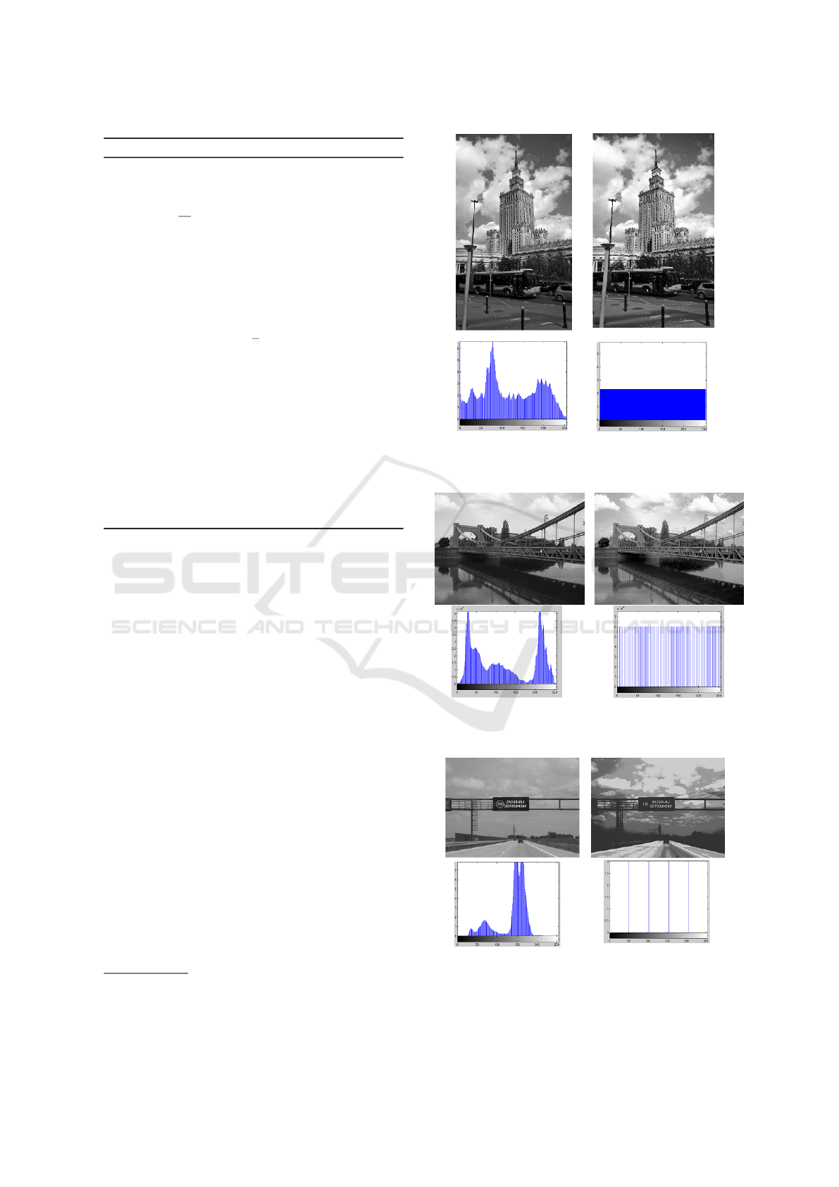
Picture Quality. Picture quality after transforma-
tion is surprisingly good in most cases. First, we
evaluated visual quality of dozens of pictures. Ex-
cept some artificial cases (e.g., monochromatic pic-
ture with all values of all pixels set to
0
0
0
), the qual-
ity of the pictures after transformation was acceptably
good. As a typical examples we present Figures 2 and
3. The picture on the left is the original; on the right
– histogram adjusted.
Numerical Analysis of Deformation. We also per-
formed a series of experiments to inspect how the pic-
ture is changed, i.e. we analyze residuum
3
|I − I
0
|.
Full results are presented in Table 7. We used 10
devices: Acer S56 (Ac), Canon SX160IS (Ca), Ko-
dak P850 (Ko), Lumia 640 (Lu), Nikon D3100 (N1),
3
A matrix |I − I
0
| containing absolute values of pixel differ-
ences between original image I and after DEPECHE trans-
form I
0
.
Figure 2: On the left: original image (256 colors), on the
right: image after transformation to 256 colors (Lumia 640).
Mean of |I − I
0
| is 11.2, the standard deviation is 6.7.
Figure 3: On the left: original image, on the right: image
after transformation to 64 colors (Samsung A40). Mean of
|I − I
0
| is 16.47, the standard deviation is 8.72.
Figure 4: On the left: original image, on the right: image
after transformation to 4 colors (Samsung A40). Mean of
|I − I
0
| is 23.33, the standard deviation is 16.08.
SECRYPT 2017 - 14th International Conference on Security and Cryptography
348

Nikon P100 (N2), Samsung A40 (S1), Samsung Ace
3 (S2), Samsung Omnia II (S3) and Samsung SIII
mini (S4). All cameras except Canon, Kodak and
Samsung A40 (CCD), have the CMOS sensor. Infor-
mation about image resolutions is presented in Table
6. The total number of 200 8-bit grayscale images
(20 per each camera) were adjusted to 4, 8, 16, 32,
64, 128 and 256 intensity levels. For each input im-
age I and adjusted image I
0
we calculated mean and
standard deviation of the difference |I − I
0
|.
Note that with all camera types, the differences be-
tween the original image I and the histogram-adjusted
image I
0
were at small level. The smallest differ-
ences were observed in case of Canon SX160IS, Lu-
mia 640 and Samsung Omnia II – the average differ-
ence of pixels intensity of I and I
0
was around 20. The
biggest differences appeared in Nikon P100 and Sam-
sung Ace 3 – about 30. However, such difference is
not easily noted visually. Sample images and their
difference are presented in Figures 2 and 3. Obvi-
ously, for 4-color image I
0
the differences between
original and adjusted image were the biggest, how-
ever even in this case the visual reception could be
regarded as satisfactory.
4 RELATED WORK
One of the most popular work on camera sensor
recognition is Lukás et al. (Lukás et al., 2006) al-
gorithm recalled in Section 2. The authors proposed
an algorithm for calculating the PRNU (Photo Re-
sponse Non Uniformity). The algorithm utilizes the
residual noise, which is defined as a difference be-
tween image p and its denoised form F(p). A typ-
ical image of size 12Mpix is processed in 3-4 min-
utes. Goljan in (Goljan, 2008) proposed a tech-
nique based on cross-correlation analysis and peak-
to-correlation-energy (PCE) ratio to identify the cam-
era. The method calculates the PRNU pattern and
uses the correlation detector with PCE ratio to mea-
sure the similarity between noise residuals. The time
performance is not examined. In (Kang et al., 2012)
a method that enhances the results in (Lukás et al.,
2006) was presented. A sensor fingerprint is consid-
ered as a white noise present on the images. The au-
thors propose to use correlation to circular correla-
tion norm as the test statistic, which can reduce the
false positive rate of camera recognition. The TPR of
recognition was 95% (images of size 256x256px) and
99% (512x512px). In (Goljan and Fridrich, 2014) a
method of identifying a camera based on parameters
of radial distortion is proposed. These parameters are
considered to be unique for each camera. Despite pos-
sible identification in some cases FAR may rise up
to 40% (and exceed 50% in case of Nikon cameras).
A comprehensive survey of image forensics methods
can be found in (Birajdar and Mankar, 2013).
In (Julliand et al., 2016) the authors show that dif-
ferent types of noise strongly affects the raw image.
It is obvious that JPEG lossy compression generates a
noise that impacts groups of pixels. A particular im-
age was presented that before saving it to the JPEG
has a different histogram than the resulting image.
Hence, JPEG compression adds some specific arti-
facts to the final image and the exact implementation
details may be used for identification. In (Taspinar
et al., 2016) it is considered, if sensor recognition can
be made when the image block is less than 50×50px.
As a verification, the Peak-to-correlation energy ratio
is used. Results showed that the efficiency of analyz-
ing so small blocks is not satisfactory and the PCE
values are low. The goal of (Jiang et al., 2016) is to
determine if images in social network in several ac-
counts were taken by the same user. The authors use
the same formula as in (Lukás et al., 2006) for find-
ing the camera fingerprint and cluster the images by
the correlation. Authors performed experiments with
1576 images and used the precision and recall mea-
sures for evaluation of the performance. The preci-
sion of clustering performance was 85%, the recall
– 42%. The impact of pixel defects as: point/hot
point defects, dead pixels, pixels traps and cluster de-
fects was investigated in (Li et al., 2014; Chapman
et al., 2015) among others. In (Lanh et al., 2007),
twelve cameras were experimentally investigated for
defected pixels and compared with each other. Re-
sults showed that each camera had a distinct pattern of
defective pixels. Therefore, in order to preserve ones
privacy, there is a need to obfuscate such defects, e.g.
by adjusting image intensity histogram.
5 CONCLUSION
In this paper we have investigated the problem of link-
ing digital cameras and its pictures. We proposed
an algorithm for tracing the camera based on peak
signal-to-noise ratio that is faster then well-known
Lukás et al. algorithm, but in some cases less accu-
rate. In the second part we introduced an algorithm
for adjusting image histogram to the uniform form.
This method hides some specific artifacts that may by
used for identifying the devices.
Both branches of the research in the paper may
be further investigated. In particular a very promis-
ing idea is replacing the uniform histogram in DE-
PECHE with Gauss-like or widely used in image anal-
ysis Rayleigh distribution.
Some Remarks about Tracing Digital Cameras – Faster Method and Usable Countermeasure
349

Table 6: Devices and image resolutions.
Ac Ca Ko Lu N1 N2 S1 S2 and S3 S4
Img 4096x2304 4608x3456 2592x1944 3264x1840 4608x3072 3648x2736 2272x1704 2560x1920 2560x1536
Sensor CMOS CCD CCD CMOS CMOS CMOS CCD CMOS CMOS
Table 7: Average difference, standard deviation and median of pixel intensities for each tested camera between image I and I
0
for adjusting the histogram to 4. 8. 16. 32. 64. 128 and 256 colors.
# of colors Ac Ca Ko Lu N1 N2 S1 S2 S3 S4
4
mean 30.52 22.40 31.59 24.02 30.73 31.88 26.74 33.56 23.94 23.19
stddev 18.11 15.32 17.62 15.05 17.95 18.00 15.83 18.52 14.37 14.97
8
mean 26.85 21.00 27.41 22.34 31.90 30.83 25.38 31.02 21.72 21.13
stddev 16.95 14.28 15.39 14.09 19.46 19.34 15.36 17.18 13.28 13.32
16
mean 25.78 22.71 26.14 21.78 31.10 31.34 26.45 31.16 21.17 22.56
stddev 17.04 14.58 15.45 14.64 21.81 21.34 16.22 18.68 13.96 14.13
32
mean 26.95 23.07 26.30 23.76 33.50 32.07 26.99 30.69 22.33 22.59
stddev 17.35 14.75 15.47 15.55 22.66 21.58 16.20 18.63 14.86 13.99
64
mean 25.55 22.56 25.88 21.45 30.95 31.25 26.32 30.99 20.92 22.32
stddev 16.69 14.20 15.04 14.36 21.56 21.12 15.85 18.48 13.63 13.80
128
mean 25.28 22.50 25.87 20.95 30.38 31.10 26.20 31.12 20.66 22.34
stddev 16.53 14.10 14.90 14.03 21.25 20.99 15.81 18.42 13.31 13.76
256
mean 25.40 22.52 25.86 21.18 30.65 31.17 26.25 31.04 20.78 22.32
stddev 16.59 14.13 14.95 14.18 21.39 21.04 15.81 18.44 13.45 13.77
REFERENCES
Birajdar, G. K. and Mankar, V. H. (2013). Digital image
forgery detection using passive techniques: A survey.
Digital Investigation, 10(3):226–245.
Chapman, G. H., Thomas, R., Thomas, R., Koren, Z., and
Koren, I. (2015). Enhanced correction methods for
high density hot pixel defects in digital imagers.
Galdi, C., Nappi, M., and Dugelay, J. (2016). Multimodal
authentication on smartphones: Combining iris and
sensor recognition for a double check of user identity.
Pattern Recognition Letters, 82:144–153.
Goljan, M. (2008). Digital camera identification from im-
ages - estimating false acceptance probability. In Digi-
tal Watermarking, 7th International Workshop, IWDW
2008, pages 454–468.
Goljan, M. and Fridrich, J. J. (2014). Estimation of lens
distortion correction from single images. In Media
Watermarking, Security, and Forensics 2014, page
90280N.
Horé, A. and Ziou, D. (2010). Image quality metrics: PSNR
vs. SSIM. In 20th International Conference on Pattern
Recognition, ICPR 2010, pages 2366–2369.
Jiang, X., Wei, S., Zhao, R., Zhao, Y., and Wu, X. (2016).
Camera fingerprint: A new perspective for identifying
user’s identity. CoRR, abs/1610.07728.
Julliand, T., Nozick, V., and Talbot, H. (2016). Image Noise
and Digital Image Forensics, pages 3–17. Springer
International Publishing, Cham.
Kang, X., Li, Y., Qu, Z., and Huang, J. (2012). Enhancing
source camera identification performance with a cam-
era reference phase sensor pattern noise. IEEE Trans.
Information Forensics and Security, 7(2):393–402.
Lanh, T. V., Chong, K., Emmanuel, S., and Kankanhalli,
M. S. (2007). A survey on digital camera image foren-
sic methods. In Proceedings of the 2007 IEEE Inter-
national Conference on Multimedia and Expo, ICME
2007, pages 16–19.
Li, X., Shen, H., Zhang, L., Zhang, H., and Yuan, Q. (2014).
Dead pixel completion of aqua MODIS band 6 using
a robust m-estimator multiregression. IEEE Geosci.
Remote Sensing Lett., 11(4):768–772.
Lukás, J., Fridrich, J. J., and Goljan, M. (2006). Digital
camera identification from sensor pattern noise. IEEE
Trans. Information Forensics and Security, 1(2):205–
214.
Lukás, J., Fridrich, J. J., and Goljan, M. (2016). Matlab
implementation.
Na, T. and Kim, M. (2014). A novel no-reference PSNR
estimation method with regard to deblocking filtering
effect in H.264/AVC bitstreams. IEEE Trans. Circuits
Syst. Video Techn., 24(2):320–330.
Tanchenko, A. (2014). Visual-psnr measure of image qual-
ity. J. Visual Communication and Image Representa-
tion, 25(5):874–878.
Taspinar, S., Mohanty, M., and Memon, N. D. (2016).
PRNU based source attribution with a collection of
seam-carved images. In 2016 IEEE International
Conference on Image Processing, ICIP 2016, pages
156–160.
SECRYPT 2017 - 14th International Conference on Security and Cryptography
350
