
Smooth Autonomous Take-off and Landing Maneuvers over a
Double-hulled Watercraft
Omar Velasco, Pablo J. Alhama Blanco and Jo
˜
ao Valente
Departamento de Ingenier
´
ıa de Sistemas y Automatica, Universidad Carlos III de Madrid, Legan
´
es, Madrid, Spain
Keywords:
Aerial-marine Robotic System, Vertical Take-off and Landing, Classic Control, Dynamic Movement Primi-
tives.
Abstract:
This paper addresses the problem of vertical take-off and landing (VTOL) over a moving target in an inland
water environment. The maneuvers are carried out by a multi-rotor unmanned aerial system (UAS) over a
double-hulled watercraft unmanned surface vehicle (USV). The approach proposed employs a cascade PID
control architecture and is then improved with Dynamic Movement Primitives (DMP). The results presented
show that DMP can be used in combination with PID classical control for achieving a more safe and accurate
VTOL maneuver.
1 INTRODUCTION
Quality assessment of inland waters is one of the
most important action fields launched by the Euro-
pean Union until 2022 for biodiversity and habitat
conservation.
The branch of science that addresses the studies of
inland aquatic ecosystems is called limnology. Wa-
ter quality evaluation is achieved through the analy-
sis and classification of different biophysical and bio-
chemical parameters. This parameters are usually ac-
quired locally with manual instrumentation close by
the water, and also through satellites or airborne im-
agery.
Manual sampling techniques have been used tra-
ditionally, but they involve tedious operations and
increase the probability of erroneous field practices.
Moreover, satellite imagery is not always available
and the spatial resolution is limited for certain appli-
cations. Finally, airborne surveys are subject to strict
legislation for flying over natural environments and
ungovernable logistics. It should also be highlighted
that all those approaches have increased associated
operation costs.
Unmanned aerial systems (UAS) have improved
remote sensing (RS) missions from different domains
by providing a personal channel of data delivery for
researcher and end-users. In this way, their usability
in limnology will also play an important role because
data may be delivered in short time windows and with
affordable operation costs.
The UAS can be successful used in aquatic en-
vironments (Ore et al., 2015), however they have a
very limited autonomy, and they might be vulnerable
to unexpected weather changes. In order to avoid ac-
cidents and damages to the platform it is important to
constantly have available an emergency landing plat-
form fot the UAS during the mission.
In this paper we present a set of control strategies
for autonomous vertical takeoff and landing (VTOL)
with a quadrotor and a double-hulled watercraft.
A multiple robot UAS-USV configuration was
presented in (Djapic et al., 2015) focusing on the im-
plementation of the control approach and the com-
munication interfaces. In (Pinto et al., 2014) a more
complex collaboration system was designed for envi-
ronmental data gathering with autonomous operation,
including VTOL. Another aerial and marine collabo-
ration using a visual servoing algorithm is presented
in (Weaver et al., ).
The work presented herein can be distinguished
by the smaller scale of the aerial platforms in the
multi-robot team. This characteristic enables rapid
deployment in areas with difficult access and hard to
survey. Moreover, a reliable path tracking controller
for smooth landing and take off sequences was de-
signed to minimize the risk of the quadcopter falling
into the water during the VTOL manoeuvres.
This paper is organized as follows: The back-
ground of the problem is firstly given. Then, the plat-
forms used, as well as the scenario, and the assump-
tions are introduced in Section 2. Section 3 explains
Velasco, O., Blanco, P. and Valente, J.
Smooth Autonomous Take-off and Landing Maneuvers over a Double-hulled Watercraft.
DOI: 10.5220/0006435303890396
In Proceedings of the 14th International Conference on Informatics in Control, Automation and Robotics (ICINCO 2017) - Volume 2, pages 389-396
ISBN: Not Available
Copyright © 2017 by SCITEPRESS – Science and Technology Publications, Lda. All rights reserved
389

how the platforms dynamic models were obtained,
followed by the control strategy applied in Section 4.
After that, DMPs are presented and used to improve
the previous control approach in Section 5. Simula-
tions results are presented in Section 6, and conclu-
sion remarks in Section 7.
2 ROBOTIC SYSTEM, SCENARIO
AND ASSUMPTIONS
This section presents the multi-robot team modelled
in this work, and covers the characteristics of the
modeling scenario.
2.1 Robotic System
The modelled aerial platform is based in the
AR.Drone quadcopter, while the USV is a built from
the scratch platform named Strider V1.0. The objec-
tive of this multi-robot solution is to provide a collab-
oration system to perform data collection tasks in rel-
atively still waters. The USV aims to provide longer
autonomy to the UAV behaving as a mobile landing
platform and charging station. The drone provides the
agility and flexibility to access zones where the USV
cannot reach.
2.2 Scenario and Assumptions
The solution presented in this work is particularly des-
tined to inland water environments where wave in-
cidence is negligible. The assumptions made during
the dynamic modeling of both vehicles will be based
upon this conditions. Therefore, angle variation in the
USV’s roll, pitch and heave are not considered.
3 DYNAMIC MODELING
This section deals with the dynamic modeling of the
two autonomous vehicles presented in this work. We
consider the UAV and the USV as single rigid body
systems to obtain the models of their dynamics. The
Newton-Euler formalism will be used to describe the
motion of both autonomous platforms.
3.1 Quad-rotor Helicopter
Concerning quadcopter modeling, an inertial and a
fixed-body frame will be defined, following the no-
tation in Figure 1, where E is the inertial earth frame,
Figure 1: Coordinate system schematic and notation for the
quadcopter motion description.
following a right handed NED coordinate system con-
vention, and B is the body-fixed frame, attached to
the quadcopter airframe and along the arms of the
quadrotor.
Let us then define the following workspace within
this two frames. Two vectors can be defined to give
a generalized overview of the position and velocity of
the quadrotor in the space:
ξ =
Γ
E
Θ
E
T
=
x
q
y
q
z
q
φ
q
θ
q
ψ
q
T
(1)
ν
q
=
V
B
ω
B
T
=
u
q
v
q
w
q
p
q
q
q
r
q
T
(2)
Where ξ [+] represents the generalized position of
the body with in terms of the earth frame and ν
q
[+]
the generalized velocity of the quad-copter in terms of
the body frame. The vector V
B
[m s
−1
] represents the
linear velocity vector of the body frame with respect
to the inertial frame, being u
q
,v
q
and ω
q
the veloc-
ities in the positive x
B
, y
B
and z
B
directions respec-
tively. Similarly, the vector ω
B
[rad s
−1
] represents
the angular velocity of the quadrotor with respect to
the inertial frame, being p
q
,q
q
and r
q
the angular ve-
locities around the x
B
, y
B
and z
B
axis. Γ
E
[m] and Θ
E
[rad] represent the linear and angular position, being
x
q
,y
q
and z
q
the position of the body frame with re-
spect to the earth frame and φ
q
stands for roll, θ
q
for
pitch and ψ
q
for yaw of the body frame with respect
to the inertial frame.
Before we delve into the expressions for the mo-
tion of the quadrotor we will set a series of assump-
tions in order to simplify this task:
1. The body-fixed frame axes coincide with the prin-
cipal axes of inertia of the body
2. The moments of inertia are constant.
3. The body-fixed frame origin o
B
is coincident with
the centre of mass.
4. Body symmetry with respect to the centre of mass
is assumed.
ICINCO 2017 - 14th International Conference on Informatics in Control, Automation and Robotics
390

5. Minor aerodynamic effects such as blade flapping
or induced drag are not considered.
Using the previously defined workspace we can
obtain an expression for the motion of the quadcopter.
Equation 3 expresses the generalized expression for
the motion of any rigid body based on the assump-
tions made before:
m
q
I
3×3
0
3×3
0
3×3
I
˙
V
B
˙
ω
B
+
ω
B
× (m
q
V
B
)
ω
B
× (Iω
B
)
=
F
B
τ
B
(3)
Where m
q
[Kg] is the mass and I [N m s
2
] is the in-
ertia matrix of the quadrotor, with respect to the body
frame, and τ
B
[N m] and F
B
[N] are the force and torque
with respect to the body frame. We can characterize
this expression to the quadcopter model by defining
the force and torque vector at the right side of the
equation. In the case of the quadcopter model, this
force and torque vector, shown in equation 4, can be
divided into four components:
F
B
τ
B
=
F
B
G
0
3×1
+ U
B
+
0
3×1
G
B
a
+ F
B
ext
(4)
Gravitational Contribution.This component comes
from the effect of gravity on the quadrotor. It can
be modelled as:
F
B
G
(Θ) = R
−1
Θ
F
E
G
= R
T
Θ
0
0
m
q
g
=
−m
q
gs(θ)
m
q
gc(θ)s(φ)
m
q
gc(θ)s(φ)
(5)
Where F
B
G
is the force vector due to the gravita-
tional contribution expressed in the body frame
and c
α
= cos(α), s
α
= sin(α).
Input Contribution. From the actuation of the four
rotors of the quadcopter. Following the typical de-
scription of the four basic basic movements of a
quadrotor, namely Throttle (U
1
), Roll (U
2
), Pitch
(U
3
) and Yaw (U
4
) this contribution can be defined
as:
U
B
=
0
0
U
1
U
2
U
3
U
4
=
0
0
−c
T
(Ω
2
1
+ Ω
2
2
+ Ω
2
3
+ Ω
2
4
)
c
T
l(Ω
2
2
− Ω
2
4
)
c
T
l(Ω
2
1
− Ω
2
3
)
c
q
(Ω
2
2
+ Ω
2
4
− Ω
2
1
− Ω
2
3
)
(6)
Where T
i
and Ω
i
are the generated thrust and
speeds of each rotor respectively, starting by
the rotor located in the x
B
axis and counting
counter-clockwise, c
T
[N s
2
] and c
q
[N m s
2
] are
the thrust and drag coefficients and l [m] is the
distance between the centre of the quadrotor and
the centre of the propeller.
Gyroscopic Effects Due to Propeller Rotation.
Due to the interaction between the rotating
elements of the quadcopter and the airframe.
The expression of this gyroscopic torque is given
by the following expression (Erginer and Altug,
2007):
G
B
a
=
4
∑
i=1
I
p
(ω
B
×e
z
)(−1)
i+1
Ω
i
∈ R
3×1
(7)
Where I
p
[N m s
2
] is the moment of inertia of the
propeller, e
z
is a unitary vector in the z
E
direction
and Ω
i
the speed of each rotor.
External and Other Forces. Comprising exogenous
forces to the quadcopter and other effects, such as
minor aerodynamic forces.
3.2 Double-hulled Watercraft
For the dynamic modeling of the Strider V1.0 a sim-
ilar rigid-body mechanical model to the one used in
the previous section is adopted. An inertial and a
body fixed frame will be defined to create a suit-
able workspace for the model. The SNAME (Society
of Naval Architects and Marine Engineers) provides
with a standard notation and sign convention for the
description of the motion of ships shown in Figure 2.
Figure 2: Standard notation and sign conventions for ship
motion description on the Strider V1.0.
Again, an inertial earth frame, following the NED
convention, and a body-fixed frame, attached to the
vehicle’s platform, are defined following the notation
shown in Figure 2. With this in mind the following
notation will be used:
η
E
=
x y z φ θ ψ
T
(8)
ν
B
=
u v w p q r
T
(9)
Λ
B
=
X Y Z K M N
T
(10)
Smooth Autonomous Take-off and Landing Maneuvers over a Double-hulled Watercraft
391

Where η
E
[+] is the linear and angular position
with respect to the inertial frame, ν
B
[+] the linear and
angular velocity of the vessel with respect to the body
frame and Λ
B
[+] represents the forces and torques ap-
plied to the vessel in terms of the body fixed frame.
In this work Manoeuvring Theory is adopted to
model our simulation. Manoeuvring Theory involves
the study of the vessel’s movement at a constant or
slowly varying positive speed. A three degrees of
freedom approach is commonly considered, where
only surge, sway and yaw are analysed since re-
stricted, calm water and still waves are assumed (Fos-
sen, 2011). The modelling approach selected in this
work, based on a three degrees of freedom (DOF) ma-
noeuvring theory, involves a set of assumptions, sum-
marized in the following list:
1. The body-fixed frame axes coincide with the prin-
cipal axes of inertia of the body
2. The moments of inertia are constant.
3. Body symmetry with respect to the centre of mass
is assumed.
4. The body-fixed frame origin O
0
is coincident with
the centre of mass.
5. Restricted, calm and still water bodies is assumed.
This implies that no currents or waves affect the
motion of the ship.
6. Heave, roll and pitch motions are neglected due to
a zero frequency wave excitation assumption.
7. Surge motion is decoupled from sway and yaw
motion due to the symmetry of the vessel hulls.
8. Added mass effects on the hulls are neglected
since only steady motion will be considered.
Now, taking from the generalized expression for the
motion of a rigid body in equation 3, still valid to the
model of the Strider V1.0 due to the made assump-
tions, we can define this 3DOF motion as:
m
v
0 0
0 m
v
0
0 0 I
z
˙u
˙v
˙r
+
0 −m
v
r 0
m
v
r 0 0
0 0 0
u
v
r
=
X
Y
N
(11)
Where m
v
[Kg] is the mass of the vessel. We can
characterize this expression to the Strider V1.0 model
by defining the forces and torques at play in the
motion of the vessel. In the case of the Strider V1.0
model, this force and torque vector can be divided
into three components:
Hydrodynamic Effects. This contribution comes
from the physical interaction of the hulls with the
water. The analytical expression for the hydrody-
namic forces is expressed in terms of the hydrody-
namic coefficients. In this work the modelling ap-
proach made by Davidson and Schiff will be used
(Davidson and Schiff, 1946):
Y = Y
v
v +Y
r
r +Y
δ
δ
R
(12)
N = N
v
v + N
r
r + N
δ
δ
R
(13)
X = X(u)+ T (14)
Where, the constant coefficients (Y
v
=
∂Y
∂v
Y
r
=
∂Y
∂r
···) represent the hydro-
dynamic derivatives, X(u) is the hydrodynamic
resistance (which is a function of the forward
speed) and T is the thrust generated by the
propeller.
Control Surfaces and Propulsion. Generated by
the control surfaces (rudder, fins, etc) and the
propulsion forces from the vessel thruster. The
propeller thrust is modelled directly as a force,
but rudder forces are analytically implemented
through the below expression (Perez and Blanke,
2002):
X
rudder
= −F
R
(u,V
av
,v, r,δ)sin(δ)
Y
rudder
= F
R
(u,V
av
,v, r,δ)cos(δ)
Z
rudder
= 0
(15)
Where F
R
is defined as:
F
R
=
1
2
ρC
L
A
r
V
2
av
sin(
π
2
δ
attack
δ
stall
) i f |δ
attack
| < δ
stall
1
2
ρC
L
A
r
V
2
av
sign(δ
attack
) i f |δ
attack
| > δ
stall
(16)
Where ρ [Kg m
−
3] is the density of the water,
C
L
[−] is the lift coefficient of the rudder, A
r
[m
2
]
is the rudder area, V
av
[m s
−2
] is the average flow
passing the rudder and δ
stall
[rad] is the stall angle
of the rudder. The function sign(k) gives back
the sign of k. The angle of attack δ
attack
[rad] is
the angle between the plane of the rudder and the
direction of the flow passing by the rudder.
External Forces. Comprising exogenous forces to
the vessel such as wind or currents or any other
external disturbance.
4 PID CONTROL
PID control techniques are the most used linear regu-
lators. This is due to their simple structure and easy
ICINCO 2017 - 14th International Conference on Informatics in Control, Automation and Robotics
392

implementation, good applicability to a wide arrange
of control problems and their tunability of ”blackbox”
systems, where the plant is not identified.
In the case of the quadrotor control system, a PID
cascade architecture has been used to obtain control
of the vehicle. Figure 3 illustrates the control archi-
tecture used in this work for the quadcopter. The
implemented architecture features three nested PID
feedback loops, each one controlling the position, ve-
locity and attitude of the quadcopter respectively.
Figure 3: Cascade loop architecture used for the control of
the quadcopter.
The control architecture of the Strider V1.0 is eas-
ier to implement than the quadrotor system since only
two degrees of freedom of the vessel will be con-
trolled. Two separate closed loop PID controllers will
command the surge speed u and the heading ψ of the
vessel through the actuation of the propeller’s thrust
and the rudder action respectively.
4.1 Trajectory Tracking
A trajectory tracking algorithm was also implemented
in the control architecture of the USV in order to per-
form planned sweeps and other autonomous path fol-
lowing tasks. Planned routes of any unmanned vehi-
cle can be represented in terms of way-points. Way-
points are defined in Cartesian coordinates (x
k
,y
k
,z
k
)
for k = 1, 2, . . . , n. and represent an ordered database
of points in the working space (Fossen, 2011):
wpt.pos = (x
0
,y
0
,z
0
),(x
1
,y
1
,z
1
),... ,(x
n
,y
n
,z
n
) (17)
One of the simplest and common methods of im-
plementing path control based on way-point trajec-
tory planing is the use of Line Of Sight(LOS) guid-
ance. LOS guidance is based on the calculation of a
straight trajectory from the current position of the ve-
hicle and the following way-point using the following
expression:
ψ
q
(t) = tan
−1
y
q
(k) − y(t)
x
q
(k) − x(t)
(18)
Where ψ
q
(t) is the desired course angle, y
q
(k) and
x
q
(k) are the next way-point coordinates and y(t) and
x(t) the current vehicle position. Once the vehicle has
reached the way-point the next way-point is selected.
For this purpose, the concept of circle of acceptance is
adopted. When the vehicle resides within the borders
of a circle of radius ρ
0
[m] the next way-point in the
database is selected. This condition is translated into
the following inequality:
[x
q
(k) − x(t)]
2
+ [y
q
(k) − y(t)]
2
≤ ρ
2
0
(19)
4.2 Vertical Take-off and Landing
Autonomous landing on a mobile platform proves to
be a difficult task because of the involved complex-
ity of precise position estimation. The usual approach
to this problem is the use of Visual Servoing for po-
sition and tracking control as works such as (Heriss
´
e
et al., 2012) show. Although a Visual Servoing ser-
voing algorithm is out of the scope of this work, the
performance of VTOL tasks with the designed con-
troller can be evaluated.
The design of the autonomous landing controller
is based on the simple flow chart shown in Figure 4.
During the approaching phase, the quadrotor is set to
track the vessel at an altitude z
∗
over the landing plat-
form. If the position error e is less than the selected
threshold e
∗
, the quadrotor is commanded to land.
Figure 4: VTOL controller flowchart.
5 DYNAMIC MOVEMENT
PRIMITIVES (DMP)
The DMPs have been chosen for improving the VTOL
maneuvers because of their ability to operate with
all robot control parameters. They are based on
nonlinear differential equations. They also provide
smooth kinematic control parameters. This is essen-
tial to perform all the movements required in a ro-
bust and autonomous way. DMPs are well suited
to manage uncertainties, uncertain situations, unfore-
seen events, unexpected events, etc. This is possible
for several reasons, first ensuring a smooth transition
from any unforeseen changes in the path target due to
sensory feedback; Second, because they provide the
framework for learning and adapting trajectories us-
ing learning and reinforcement algorithms; Thirdly, to
allow the learning of all types of trajectories based on
one or more of a given trajectory; and lastly because
they do not explicitly depend on time.
Smooth Autonomous Take-off and Landing Maneuvers over a Double-hulled Watercraft
393

5.1 Control Parameters as Dynamic
Systems
In this section is presented the theoretical founda-
tions of the motor representation developed accord-
ing to (Ijspeert et al., 2003) and (Schaal et al., 2005).
This documents deals with the discrete DMPs that en-
code discrete point-to-point motion control parame-
ters. For rhythmic DMPs, (Ijspeert et al., 2003) and
(Gams et al., 2009) can be consulted. A DMP path
with one degree of freedom is defined by (Ijspeert
et al., 2013) with the following nonlinear differential
equations:
τ˙z
D
= α
z
D
(β
z
D
(g − y
D
) − z
D
) + f (x
D
), (20)
τ ˙y
D
= z
D
, (21)
τ ˙x
D
= −α
x
D
x
D
, (22)
Where: x
D
is the phase variable and z
D
is an auxil-
iary variable that represents the velocity, its derivative
is ˙z
D
. Moreover, β
z
D
, α
z
D
and α
x
D
are damping con-
stants, where α
z
D
= 4β
z
D
. The τ > 0 is constant, as a
temporal scaling factor. Their values are determined
in order to ensure the convergence of the system dy-
namics. This set of differential equations has a unique
attractor point y
D
= g (goal) with z
D
= 0. Finally,
f (x
D
) is defined as a linear combination of nonlinear
radial basis functions, which allow the robot to follow
a smooth path from the initial position y
D0
, to the final
configuration g.
f (x
D
) =
∑
M
i=1
w
i
Ψ
i
(x
D
)
∑
M
i=1
Ψ
i
(x
D
)
x
D
(g − y
D0
), (23)
Ψ
i
(x
D
) = exp(−h
i
(x
D
− c
i
)
2
), (24)
Where c
i
is the center of the Gaussian distribution
along the path phase and h
i
is its width. For a given
M and considering the time constant τ = τ
T
can be
defined c
i
= exp(−α
x
D
i−1
M−1
), h
i
=
1
(c
i+1
−c
i
)
2
,
h
M
= h
M−1
, i = 0,...,M. For each degree of freedom
in the cartesian space, the weight w
i
is estimated by
the measured data and using a regression according
to (Nemec et al., 2009), g being he last configuration
saved during the trajectory. In this way the desired tra-
jectory is obtained. Since discrete DMPs have been
designed to represent discrete point-to-point move-
ments, the motion must pass smoothly and continu-
ously at the end of the path, that is, at time τ
T
.
0 2 4 6 8 10 12
t (s)
-1.2
-1
-0.8
-0.6
-0.4
-0.2
0
0.2
X position (m)
P1 Lon Cmd
P2 Lon Cmd
P1 Measured Lon
P2 Measured Lon
Figure 5: Longitude commands and measured values during
the test.
0 2 4 6 8 10 12
t (s)
0
0.2
0.4
0.6
0.8
1
Lon position error (m)
P1 Lon position error
P2 Lon position error
Figure 6: Longitude position errors during the test.
6 EXPERIMENTS
This section will present the results obtained from the
simulation of several tests to evaluate the performance
of the designed controller.
6.1 Way-point Guidance Test
Way-point guidance was implemented for position
control of the Strider V1.0. Several tests were per-
formed with different path setups. Starting from the
coordinates origin, a constant speed of 1 m/s was
commanded to the vessel since this is the reference
speed used for the dynamic modeling of the forces.
Further analysis and results of the performance of this
controller can be found in (Omar, 2017).
6.2 DMP in Path Tracking Controllers
In this part, the performance of the proposed method
of improving a classic control with dynamic move-
ment primitives is evaluated. The base of experiments
is centered on three scenarios. A first base scenario
P1 in which a control based on a cascade PID con-
trol architecture is performed. A second scenario P2
in which changes are introduced by the use of DMPs.
Finally a third scenario P3, where it is compared with
the case in which the operator handles the quadcopter
manually. One of the characteristics of the DMP
is the smoothness in the reproduction of movements.
For a smooth movement during the course of the tra-
ICINCO 2017 - 14th International Conference on Informatics in Control, Automation and Robotics
394

0 2 4 6 8 10 12
t (s)
0
0.5
1
1.5
2
Lat (m)
P1 Lat Cmd
P2 Lat Cmd
P1 Measured Lat
P2 Measured Lat
Figure 7: Latitude commands and measured values during
the test.
0 2 4 6 8 10 12
t (s)
0
0.2
0.4
0.6
0.8
1
1.2
Lat position error (m)
P1 Lat position error
P2 Lat position error
Figure 8: Latitude position errors during the test.
jectory, a treatment of the Cartesian control param-
eters is carried out using the UAV dynamic model.
Within the analyzed parameters we can highlight the
VTOL performance of the scenarios P1 and P2. Con-
cerning the path tracking performance, Figures 7 and
5 illustrate the system’s path tracking response during
tests P1 and P2. The position errors of the quadro-
tor during flight are shown in 8 and 6. These errors
represent the distance between the original position
command (that of P1) and the measured latitude and
longitude during both tests. Another parameter ana-
lyzed is the settling time of the controller. As it can
be seen from the results in the figures, especially from
the analysis of the error plots, the results from P2
show a quicker settling time, which overall results in
a smaller average position error during the test. This
behavior, although more aggressive than P1 in some
cases (where the error from P2 is bigger than the error
from P1) provides a more tight path following perfor-
mance, which heavily benefits autonomous take off
and landing duties. Regarding the behavior against
overshoots, it is where more significant improvements
are obtained, In figure 9 it is possible to see in a dy-
namic way the abrupt changes made by the operator
of the scenario P3. In front of a soft control param-
eters thanks to the DMP. Despite of being a very in-
cipient experimentation it can be said that the prelimi-
nary results are satisfactory. It is intended to continue
to introduce characteristics of the DMP, such as the
treatment of rhythmic movements in surveying duties
(a typical task for drones) or dynamic evasion of ob-
stacles during VTOL.
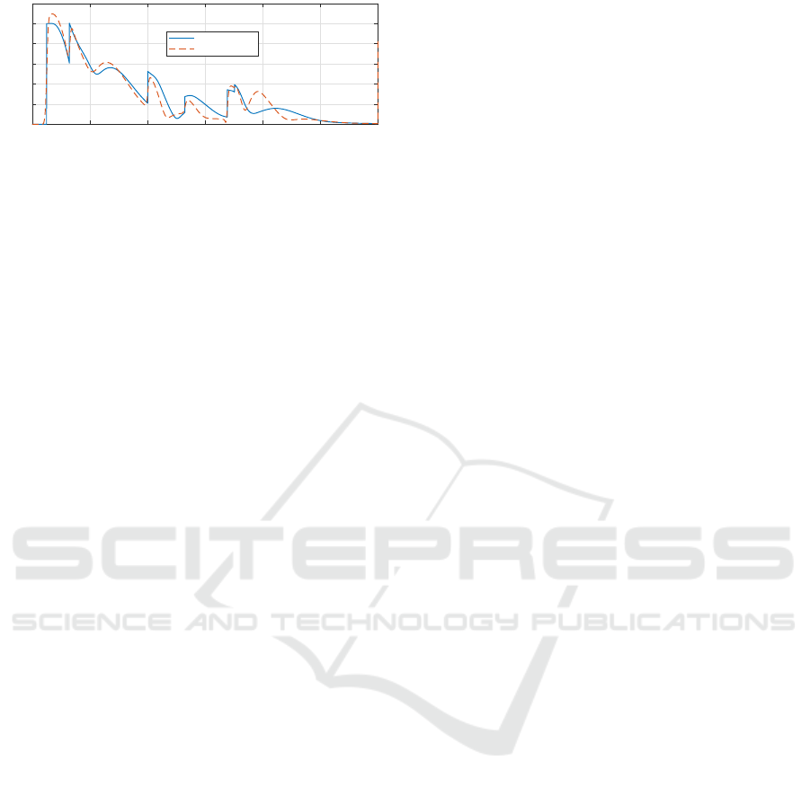
Figure 9: Comparative between operator and DMPs.
1 2 3 4 5 6 7 8 9 10
t (s)
0
0.5
1
1.5
2
Altitude(m)
VTOL performance
P1 Altitude Command
P1 Altitude
P2 Altitude Command
P2 Altitude
Figure 10: Height values during P1 and P2 testing.
6.3 DMPs and VTOL Tests
We will evaluate the performance of the VTOL and
tracking algorithm comparing the two scenarios P1
and P2. The quadrotor is set to track the position of
the moving landing platform. It autonomously takes
off at the start of the test (t = 0s) and then the VTOL
controller is activated at 5,5 seconds and set to land-
ing mode. The controller parameters, from Figure 4,
used for the test were e
∗
= 0.12 m and h
∗
= 0.3 m.
Figure 10 shows the height measured values and
command of the quadrotor during tests P1 and P2.
The three phases of the algorithm can be easily iden-
tified by seeing the commanded height values during
the test, where the three height command levels rep-
resent each of the states of the controller respectively.
Figure 11 presents the absolute position error, repre-
senting the distance from the quadrotor to the cen-
tre of the landing pad. As it can be seen from both
figures, the performance of the DMP path tracking
(P2) yields a much smoother landing sequence. This
is thanks to the benefits of the DMP, since the abso-
lute error gets reduced into the minimum landing er-
ror threshold.
It can be seen that the VTOL algorithm functions
properly and that the quadcopter is able to safely
land in the platform within the error constrains that
were set in both tests, however when treating the path
tracking controller with DMP the results provide with
lower landing times, reducing the inherent possibility
of hazard during this complicated manoeuvre, and a
more fluid landing behaviour.
Smooth Autonomous Take-off and Landing Maneuvers over a Double-hulled Watercraft
395
0 2 4 6 8 10 12
t (s)
0
0.2
0.4
0.6
0.8
1
1.2
Absolute position error (m)
P1 absolute error
P2 absolute error
Figure 11: Absolute position error of the quadcopter during
the VTOL test.
7 CONCLUSIONS
The approach proposed in this work shows how to im-
prove a classic control system dedicated to VTOL op-
erations over a moving target. In particular its shown
that the trajectory tracking error might be improved
and the UAS is able to perform a smooth VTOL ma-
noeuvre over the USV.
The stability and softness provided by the dy-
namic movement primitives might be able to improve
navigation manoeuvres subject to waves or even with
wind gusts, and including dynamic obstacle avoid-
ance capabilities. In spite of the early characteristic
of this experimentation, the preliminary results hint
of a sizeable improvement once more characteristics
of the DMP are introduced into the control architec-
ture.
Better performance could be expected, especially
when performing repetitive cyclic and rhythmical
tasks, typical in UAS based sensing techniques.
ACKNOWLEDGMENTS
The research leading to these results has received
funding from the RoboCity2030-III-CM project
(Rob
´
otica aplicada a la mejora de la calidad de vida
de los ciudadanos. fase III; S2013/MIT-2748), funded
by Programas de Actividades I+D en la Comunidad
de Madrid and cofunded by Structural Funds of the
EU.
REFERENCES
Davidson, K. and Schiff, L. (1946). Turning and course
keeping qualities of ships. Transactions of SNAME,
4:49.
Djapic, V., Prijic, C., and Bogartz, F. (2015). Autonomous
takeoff landing of small uas from the usv. In OCEANS
2015 - MTS/IEEE Washington, pages 1–8.
Erginer, B. and Altug, E. (2007). Modeling and pd control
of a quadrotor vtol vehicle. In 2007 IEEE Intelligent
Vehicles Symposium, pages 894–899.
Fossen, T. I. (2011). Handbook of marine craft hydrody-
namics and motion control. John Wiley & Sons.
Gams, A., Ijspeert, A. J., Schaal, S., and Lenar
ˇ
ci
ˇ
c, J.
(2009). On-line learning and modulation of periodic
movements with nonlinear dynamical systems. Au-
tonomous robots, 27(1):3–23.
Heriss
´
e, B., Hamel, T., Mahony, R., and Russotto, F.-X.
(2012). Landing a vtol unmanned aerial vehicle on a
moving platform using optical flow. IEEE Transac-
tions on Robotics, 28(1):77–89.
Ijspeert, A. J., Nakanishi, J., Hoffmann, H., Pastor, P., and
Schaal, S. (2013). Dynamical movement primitives:
learning attractor models for motor behaviors. Neural
computation, 25(2):328–373.
Ijspeert, A. J., Nakanishi, J., and Schaal, S. (2003). Learn-
ing attractor landscapes for learning motor primitives.
Advances in neural information processing systems,
pages 1547–1554.
Nemec, B., Tamo
ˇ
si
¯
unait
˙
e, M., W
¨
org
¨
otter, F., and Ude, A.
(2009). Task adaptation through exploration and ac-
tion sequencing. In Humanoid Robots, 2009. Hu-
manoids 2009. 9th IEEE-RAS International Confer-
ence on, pages 610–616. IEEE.
Omar, V. A. (2017). Modelling and control of a uav-usv
collaboration scheme for fluvial operations. Bache-
lor’s thesis, Univ. Carlos III de Madrid.
Ore, J.-P., Elbaum, S., Burgin, A., Zhao, B., and Detweiler,
C. (2015). Autonomous Aerial Water Sampling, pages
137–151. Springer International Publishing, Cham.
Perez, T. and Blanke, M. (2002). Mathematical ship mod-
elling for control applications. Ørsted-DTU, Automa-
tion.
Pinto, E., Santana, P., Marques, F., Mendonc¸a, R.,
Lourenc¸o, A., and Barata, J. (2014). On the design
of a robotic system composed of an unmanned surface
vehicle and a piggybacked vtol. In Doctoral Confer-
ence on Computing, Electrical and Industrial Systems,
pages 193–200. Springer.
Schaal, S., Peters, J., Nakanishi, J., and Ijspeert, A. (2005).
Learning movement primitives. In Robotics Research.
The Eleventh International Symposium, pages 561–
572. Springer.
Weaver, J. N., Frank, D. Z., Schwartz, E. M., and Arroyo,
A. A. Uav performing autonomous landing on usv
utilizing the robot operating system.
ICINCO 2017 - 14th International Conference on Informatics in Control, Automation and Robotics
396
