
Conditional Synchronized Diagnoser for Modular Discrete-Event
Systems
Felipe G. Cabral, Maria Z. M. Veras and Marcos V. Moreira
COPPE-Electrical Engineering Program, Universidade Federal do Rio de Janeiro,
Cidade Universi
´
aria, Ilha do Fund
˜
ao, Rio de Janeiro, 21.945-970, RJ, Brazil
Keywords:
Failure Diagnosis, Modular Systems, Automata, Petri Nets.
Abstract:
In general, systems are formed by the composition of several modules, and may exhibit a large number of
states. The growth of the global system model with the number of components leads to a high computational
cost for diagnosis techniques. In order to circumvent this problem, in a recent work, a diagnosis scheme based
on the observation of the nonfailure behavior model of the system components, and their synchronization
due to observable events, is proposed. Although the computation of the global system model for diagnosis is
avoided, the estimated observed nonfailure language in this scheme can be a larger set than the actual observed
nonfailure language of the system, which leads to the notion of synchronous diagnosability. This scheme is
implemented using a diagnoser, called synchronized Petri net diagnoser (SPND). In this work, we propose the
addition of conditions for the observable transitions of the SPND, leading to a conditional synchronized Petri
net diagnoser (CSPND). We show that the addition of such conditions can cause a decrease in the observed
nonfailure language, and systems that are not synchronously diagnosable can be conditionally synchronously
diagnosable, and the delay bound can be smaller than using the synchronous diagnosis scheme.
1 INTRODUCTION
Several works in the literature address the problem
of failure diagnosis of discrete-event systems (DESs)
(Sampath et al., 1995; Sampath et al., 1996; Qiu and
Kumar, 2006; Carvalho et al., 2011; Carvalho et al.,
2012; Basilio et al., 2012; Fanti et al., 2013; Cabasino
et al., 2010; Cabasino et al., 2013; Carvalho et al.,
2013; Zaytoon and Lafortune, 2013; Cabral et al.,
2015b; Tomola et al., 2016; Santoro et al., 2017). In
the seminal work (Sampath et al., 1995), a centralized
diagnoser for DESs, constructed based on the plant
model, is proposed. However, in general, systems
are formed by the parallel composition of several sub-
systems, local components or modules, and the state
space of the plant model grows, in the worst-case, ex-
ponentially with its number of subsystems. In order
to avoid the use of the global plant model for diagno-
sis, several failure diagnosis schemes that take advan-
tage of the modularity of systems have been proposed
in the literature (Debouk et al., 2002; Contant et al.,
2006; Zhou et al., 2008; Kan John et al., 2010). In
these works, different modular diagnosability defini-
tions are introduced and local diagnosers are proposed
to detect the occurrence of failure events. The diagno-
sis decision of the global system is determined based
solely on the observations of the failure module.
In (Garc
´
ıa et al., 2006), a different approach for
modular diagnosis is proposed. Differently from (De-
bouk et al., 2002; Contant et al., 2006; Zhou et al.,
2008; Kan John et al., 2010), the method presented
in (Garc
´
ıa et al., 2006) consists of splitting the global
plant model into subsystems, constructing a minimum
controller for each subsystem, and then constructing
a local diagnoser for each subsystem composed with
its minimum controller. In (Schmidt, 2013), an in-
cremental abstraction-based approach for the verifi-
cation of modular language diagnosability of DESs is
proposed, and the differences between the online di-
agnosis methods presented in (Debouk et al., 2002;
Contant et al., 2006; Zhou et al., 2008) are reviewed.
More recently, in (Cabral et al., 2015a; Cabral
and Moreira, 2017), a new approach for online fail-
ure diagnosis of modular DESs modeled as automata
is proposed. Differently from (Debouk et al., 2002;
Contant et al., 2006; Zhou et al., 2008; Garc
´
ıa et al.,
2006; Kan John et al., 2010), a centralized synchro-
nized Petri net diagnoser (SPND) is proposed. The
SPND is formed by Petri net observers, constructed
from the nonfailure behavior models of the system
88
Cabral, F., Veras, M. and Moreira, M.
Conditional Synchronized Diagnoser for Modular Discrete-event Systems.
DOI: 10.5220/0006435700880097
In Proceedings of the 14th International Conference on Informatics in Control, Automation and Robotics (ICINCO 2017) - Volume 2, pages 88-97
ISBN: Not Available
Copyright © 2017 by SCITEPRESS – Science and Technology Publications, Lda. All rights reserved

components, and provides a superset of the state es-
timate of the global system. The Petri net observers
are naturally synchronized by the observable events
executed by the plant, and if the observation of a trace
is not recognized in the SPND, i.e., if the observa-
tion of a trace executed by the system does not be-
long to the nonfailure behavior of at least one com-
ponent of the system, the occurrence of the failure
event is indicated by using a failure detection logic. In
(Cabral et al., 2015a; Cabral and Moreira, 2017), the
authors show that if two or more components have
unobservable events in common, then the estimated
nonfailure observed language can be a larger set then
the actual observable nonfailure language of the sys-
tem. This fact can increase the delay bound for syn-
chronous diagnosis compared with the traditional di-
agnosis scheme or, in the worst-case, the failure event
is not synchronously diagnosable.
In this work, we propose a modification in the
Petri net observers that form the SPND. This mod-
ification relies on the addition of conditions to the
transitions of the Petri net observers, such that if an
event is observed by the diagnoser, the Petri net ob-
servers update their state estimate only if the occur-
rence of the event is possible in the nonfailure model
of the global system, leading to the conditional syn-
chronized Petri net diagnoser (CSPND). If an event is
observed, and the transitions labeled with this event
cannot occur in the nonfailure behavior model of the
system, then the failure event has certainly occurred,
and it is diagnosed by the CSPND. In this diagnosis
scheme, the estimated observed nonfailure language
can be a smaller set than the estimated observed non-
failure language obtained by using the synchronous
diagnosis scheme. In addition, in the worst-case, a
modular system can be conditionally synchronously
diagnosable and not synchronously diagnosable. In
this regard, we introduce the definition of conditional
synchronous diagnosability of the language of a mod-
ular system with respect to the languages of its mod-
ules. The verification of this property can be done
by using the algorithm proposed in (Cabral et al.,
2015a; Cabral and Moreira, 2017). An example is
used throughout the paper to illustrate our results.
This paper is organized as follows. In Section 2,
we present some preliminary concepts, including the
definitions of synchronous diagnosability of modular
DESs and synchronized Petri net diagnoser (SPND).
In Section 3, we present the conditional synchronized
Petri net diagnoser (CSPND). Finally, in Section 4,
the conclusions are drawn.
2 PRELIMINARIES
2.1 Notation and Definitions
Let G = (Q,Σ, f ,Γ, q
0
) denote the automaton model
of a DES, where Q is the state-space, Σ is the finite
set of events, f : Q × Σ
?
→ Q is the transition func-
tion, where Σ
?
is the Kleene-closure of Σ, Γ : Q → 2
Σ
is the feasible event function, and q
0
is the initial state
of the system. For the sake of simplicity, the feasi-
ble event function will be omitted unless stated other-
wise. The language generated by G, L(G), is denoted
in this paper by L. The accessible part of G, denoted
by Ac(G) is obtained as usual (Cassandras and Lafor-
tune, 2008).
Let G
1
and G
2
be two automata. Then, G
1
× G
2
and G
1
kG
2
denote the product and the parallel com-
position of G
1
and G
2
, respectively (Cassandras and
Lafortune, 2008).
The projection operation P
l
s
: Σ
?
l
→ Σ
?
s
, where Σ
s
⊂
Σ
l
is defined as P
l
s
(ε) = ε, P
l
s
(σ) = σ, if σ ∈ Σ
s
or
P
l
s
(σ) = ε, if σ ∈ Σ
l
\ Σ
s
, where \ denotes set dif-
ference, and P
l
s
(sσ) = P
l
s
(s)P
l
s
(σ), for all s ∈ Σ
?
l
, and
σ ∈ Σ
l
. The projection can also be applied to language
L, by applying the projection to all traces s ∈ L. The
inverse projection P
l
−1
s
: Σ
?
s
→ 2
Σ
?
l
when applied to a
trace s ∈ Σ
?
s
generates all traces of Σ
?
l
whose projec-
tion is equal to s. The inverse projection can also be
applied to languages.
Let us now suppose that the event set of G is
partitioned as Σ = Σ
o
˙
∪ Σ
uo
, where Σ
o
and Σ
uo
de-
note, respectively, the set of observable and unobserv-
able events, and let Σ
f
⊆ Σ
uo
denote the set of fail-
ure events. In this paper, we assume, without loss
of generality, that there is only one failure event, i.e.,
Σ
f
= {σ
f
}.
Definition 1. (Failure and normal traces) A failure
trace is a sequence of events s such that σ
f
is one of
the events that form s. A normal trace, on the other
hand, does not contain the event σ
f
.
The normal language L
N
⊂ L denotes the set of all
normal traces of L, and the subautomaton of G that
generates L
N
is denoted by G
N
. Thus, the set of all
traces generated by the system that contain σ
f
is L
F
=
L \ L
N
.
Let P
o
: Σ
?
→ Σ
?
o
be a projection. Then, it is
always possible to obtain a deterministic automa-
ton whose generated language is equal to P
o
(L).
This automaton is the observer of G, denoted by
Obs(G,Σ
o
) = (Q
obs
,Σ
o
, f
obs
,Γ
obs
,q
0,obs
) (Cassandras
and Lafortune, 2008).
A Petri net is another formalism usually used to
model a DES (Cassandras and Lafortune, 2008; Davi
Conditional Synchronized Diagnoser for Modular Discrete-event Systems
89

and Alla, 2005). Let N = (P,T,Pre,Post, x
0
) denote
a Petri net where P is the set of places, T is the set of
transitions, Pre : (P × T ) → N is the function of arcs
that connect places to transitions, Post : (T × P) →
N is the function of arcs that connect transitions to
places, and x
0
: P → N is the initial marking of the
system.
The set of places is denoted here by P =
{p
1
, p
2
,. . . , p
n
} and the set of transitions by T =
{t
1
,t
2
,. . . ,t
m
}. Thus, |P| = n and |T | = m, where |.|
denotes cardinality. The set of input places (resp.,
transitions) of a transition t
j
∈ T (resp., place p
i
∈ P)
is denoted by I(t
j
) (resp., I(p
i
)), and is formed by
the places p
i
∈ P (resp., transitions t
j
∈ T ) such that
Pre(p
i
,t
j
) > 0 (resp., Post(t
j
, p
i
) > 0).
The number of tokens assigned to a place p
i
is
represented by x(p
i
), where x : P → N. Thus, the
marking of a Petri net is given by the vector x =
[x(p
1
) x(p
2
) . . . x(p
n
)]
T
formed with the number of
tokens of each place p
i
, for i = 1,. . ., n. A place p
i
∈ P
is said to be safe if x(p
i
) ≤ 1 for all reachable mark-
ings of the Petri net.
A transition t
j
is said to be enabled when x(p
i
) ≥
Pre(p
i
,t
j
), ∀p
i
∈ I(t
j
). If a transition t
j
is enabled for
a marking x, then t
j
can fire reaching a new marking
¯x. The evolution of the markings is given by:
¯x(p
i
)=x(p
i
)−Pre(p
i
,t
j
)+Post(t
j
, p
i
),i = 1, . . ., n.
(1)
A binary Petri net can be defined as a Petri net
with a different evolution rule for the place mark-
ings reached after the firing of a transition t
j
given
by (Alayan and Newcomb, 1987):
¯x(p
i
) =
0,if x(p
i
)−Pre(p
i
,t
j
)+Post(t
j
, p
i
) = 0
1,if x(p
i
)−Pre(p
i
,t
j
)+Post(t
j
, p
i
) > 0
,
(2)
for i = 1,. . . , n. Notice that in a binary Petri net all
places are forced to be safe.
In order to model DESs, events are associated
with transitions in the Petri net, leading to the so-
called labeled Petri net. A labeled Petri net is
the seven-tuple N
l
= (P,T, Pre, Post, x
0
,Σ, l), where
(P,T, Pre,Post, x
0
) is a Petri net, Σ is the set of events
used to label transitions, and l : T → 2
Σ
is the transi-
tion labeling function that associates a subset of Σ to
a transition in T . An enabled transition t
j
in a labeled
Petri net fires when one of the events associated to t
j
occurs.
2.2 Diagnosability of Discrete-Event
Systems
The following definition of language diagnosability
can be stated (Sampath et al., 1995).
Definition 2. Let L and L
N
⊂ L be the live and prefix-
closed languages generated by G and G
N
, respec-
tively. Then, L is said to be diagnosable with respect
to projection P
o
: Σ
?
→ Σ
?
o
and Σ
f
if
(∃z ∈ N)(∀s ∈ L \ L
N
)(∀st ∈ L \ L
N
,ktk ≥ z) ⇒
(P
o
(st) 6∈ P
o
(L
N
)),
where k.k denotes the length of a trace.
According to Definition 2, L is diagnosable with
respect to P
o
and Σ
f
if, for all failure traces st with
arbitrarily long length after the occurrence of a fail-
ure event, there does not exist a normal trace s
N
∈ L
N
,
such that P
o
(st) = P
o
(s
N
). Therefore, if L is diagnos-
able, then it is always possible to identify the occur-
rence of a failure event after a bounded number of
observations of events.
A polynomial-time algorithm to verify language
diagnosability is presented in (Moreira et al., 2011).
2.3 Synchronous Diagnosability of
Modular Discrete-Event Systems
In (Cabral et al., 2015a; Cabral and Moreira, 2017),
the definition of synchronous diagnosability of a mod-
ular DES is presented. In order to do so, it is as-
sumed that the system is composed of r modules G
k
,
k = 1, . . . ,r, i.e., the plant G = k
r
k=1
G
k
. It is also as-
sumed that the event set of each module G
k
can be
partitioned as Σ
k
= Σ
k,o
˙
∪Σ
k,uo
, where Σ
k,o
and Σ
k,uo
denote, respectively, the sets of observable and unob-
servable events of G
k
. Moreover, each component has
its nonfailure behavior modeled by automaton G
N
k
,
such that the nonfailure behavior of the plant is given
by G
N
= k
r
k=1
G
N
k
. The main idea in (Cabral et al.,
2015a; Cabral and Moreira, 2017) is to implement
observers for each normal part of the modules of the
system, which are naturally synchronized with the ob-
servable events executed by the plant, and then, using
a failure detection logic, identify the occurrence of a
failure event. The following definition can be stated.
Definition 3. Let L and L
N
⊂ L be the languages gen-
erated by G and G
N
, respectively, and let L
F
= L\L
N
.
Consider that the system G is composed of r mod-
ules, such that G
N
= k
r
k=1
G
N
k
, where G
N
k
is the au-
tomaton that models the normal behavior of G
k
, and
let L
N
k
denote the language generated by G
N
k
, for
k = 1,. . . , r. Then, L is said to be synchronously
diagnosable with respect to L
N
k
, P
k
: Σ
?
→ Σ
?
k
, for
k = 1, .. ., r, P
o
: Σ
?
→ Σ
?
o
, and Σ
f
if
(∃z ∈ N)(∀s ∈ L
F
)(∀st ∈ L
F
,ktk ≥ z) ⇒
(P
o
(st) 6∈ ∩
r
k=1
P
o
(P
−1
k
(L
N
k
))).
ICINCO 2017 - 14th International Conference on Informatics in Control, Automation and Robotics
90

Notice that Definition 3 of synchronous diagnos-
ability of a language L is equivalent to the stan-
dard definition of diagnosability (Definition 2) of
a language L
a
= L
F
∪ L
N
a
, where L
N
a
is such that
P
o
(L
N
a
) = ∩
r
k=1
P
o
(P
−1
k
(L
N
k
)).
It is important to remark that since P
o
(L
N
a
) ⊇
P
o
(L
N
), then diagnosability is a necessary condition
for synchronous diagnosability, but it is not suffi-
cient, i.e., a system can be diagnosable but not syn-
chronously diagnosable. Moreover, since P
o
(L
N
a
) ⊇
P
o
(L
N
), the delay bound for synchronous diagnosis
can be greater that the delay bound for diagnosis. In
(Cabral et al., 2015a; Cabral and Moreira, 2017) it
is also shown that if there do not exist unobservable
events in common between the components, i.e., if
Σ
i,uo
∩ Σ
j,uo
=
/
0 for all i, j ∈ {1,. . . , r}, and i 6= j,
then P
o
(L
N
) = P
o
(L
N
a
), and diagnosability becomes
a necessary and sufficient condition for synchronous
diagnosability.
2.4 Synchronous Diagnosability
Verification
In (Cabral et al., 2015a; Cabral and Moreira, 2017),
a method for the verification of synchronous diagnos-
ability of modular discrete event systems is proposed.
The method is based on the comparison between au-
tomaton G
R
N
, whose observable language is equal to
P
o
(L
N
a
), and G
F
, that models the failure behavior of
the system G. Automaton G
R
N
is constructed in two
steps: (i) compute automata G
R
N
k
from automata G
N
k
by renaming its unobservable events using function
R
k
: Σ
N
k
→ Σ
R
N
k
, defined as:
R
k
(σ) =
σ, if σ ∈ Σ
k,o
σ
R
k
, if σ ∈ Σ
k,uo
, (3)
and; (ii) compute G
R
N
= k
r
k=1
G
R
N
k
.
In the synchronous diagnosis scheme, the syn-
chronization of unobservable events of the system
modules is lost, which leads to the possible growth of
the estimated normal language by using this scheme.
In order to model the observation of this augmented
language, the unobservable events of the normal
behavior automaton models of the system compo-
nents G
N
k
are renamed using the renaming function
(3), which leads to automata G
R
N
k
. Thus, since the
unobservable events of G
R
N
k
are private events, for
k ∈ {1, . .. , r}, the observed language of automaton
G
R
N
= k
r
k=1
G
R
N
k
models the observation of the aug-
mented normal language for synchronous diagnosis,
i.e., P
o
(L
N
a
) = P
R
o
(L(G
R
N
)), where P
R
o
: Σ
R
N
→ Σ
o
, with
Σ
R
N
= ∪
r
k=1
Σ
R
N
k
.
According to Definition 3, in order to verify if the
language L of a modular system is synchronously di-
agnosable, it is necessary to verify if the projection
P
o
: Σ
?
→ Σ
?
o
of any failure trace st, with arbitrarily
long length after the occurrence of the failure event
σ
f
, belongs to P
o
(L
N
a
). If the answer is yes, than L
is not synchronously diagnosable with respect to L
N
k
,
P
k
: Σ
?
→ Σ
?
k
, for k = 1,. .. ,r, P
o
: Σ
?
→ Σ
?
o
, and Σ
f
.
Thus, the synchronous diagnosability verification is
carried out by comparing automaton G
R
N
with the fail-
ure behavior automaton G
F
. Automaton G
F
is ob-
tained from G following the algorithm proposed in
(Moreira et al., 2011). The event set of G
F
is Σ, and
its states are labeled with N or F, such that if a state
of G
F
has the label F, then this state is reachable after
the occurrence of the failure event σ
f
.
Since the unobservable events of G
R
N
= k
r
k=1
G
R
N
k
are private events with respect to G
F
, and since
P
o
(L
N
a
) = P
R
o
(L(G
R
N
)), the verification of syn-
chronous diagnosability can be done by searching for
cyclic paths in G
V
= G
R
N
kG
F
formed by states labeled
with F and with at least one event from Σ. The lan-
guage L is synchronously diagnosable if and only if
there does not exist a cyclic path with these charac-
teristics in G
V
. In the sequel, we present an example
that illustrates the synchronous diagnosability verifi-
cation.
Example 1. Consider the system G = G
1
kG
2
, where
G
1
and G
2
are depicted in Figure 1. The set of
events of G
1
and G
2
are Σ
1
= {a, c, e,g,σ
u
} and Σ
2
=
{e,h, σ
u
,σ
f
}, where Σ
1,o
= {a,c, e,g}, Σ
2,o
= {e,h},
Σ
1,uo
= {σ
u
}, Σ
2,uo
= {σ
u
,σ
f
}, and σ
f
is the fail-
ure event. In Figures 2 and 3, we present automata
G
N
and G
F
, respectively, obtained by following the
method presented in (Moreira et al., 2011). Automa-
ton G is equal to automaton G
F
, except for the labels
N and F. In order to verify the synchronous diagnos-
ability, it is necessary to obtain the automaton models
of the normal behavior of the components of the sys-
tem G
N
1
and G
N
2
, which can be seen in Figure 4. In
the sequel, automata G
R
N
1
and G
R
N
2
, depicted in Figure
5, are computed by applying the renaming function
(3) to automata G
N
1
and G
N
2
, respectively. Automa-
ton G
R
N
= G
R
N
1
kG
R
N
2
, whose observed generated lan-
guage is P
R
o
(L(G
R
N
)) = P
o
(L
N
a
), is shown in Figure
6.
Notice that the gray states of G
R
N
do not belong
to G
N
and, thus, all observable transitions related to
such states can contribute to the growth of the esti-
mated normal language obtained by using the syn-
chronous diagnosis scheme. Finally, in order to ver-
ify the synchronous diagnosability of the system G, it
is necessary to compute the verifier automaton G
V
=
G
R
N
kG
F
and search for cyclic paths formed by states
with the label F and at least one event σ ∈ Σ. Since in
G
V
there is a cyclic path that violates the synchronous
Conditional Synchronized Diagnoser for Modular Discrete-event Systems
91

0 1
a
2
3
g
σ
u
c
e
e
σ
u
4
(a) G
1
0 1
h
2
e
σ
u
3
4
σ
f
σ
u
e
h, e
(b) G
2
Figure 1: Automata G
1
and G
2
of Example 1.
0,0,N
a
h
a
1,0,N
1,1,N0,1,N
h
σ
u
2,2,N 3,3,N
σ
u
c
4,2,N
g
3,2,N
e
e
Figure 2: Automaton G
N
of Example 1.
diagnosability condition, L is not synchronously diag-
nosable. It is important to notice that, according to
Definition 2, L is diagnosable.
2.5 Synchronized Petri Net Diagnoser
In order to implement the synchronous diagnosis
scheme, in (Cabral et al., 2015a; Cabral and Mor-
eira, 2017), the authors propose a synchronized Petri
net diagnoser (SPND). The SPND is a centralized di-
agnoser, consisting of r Petri net state observers that
provide the state estimate of the normal behavior of
the system components G
N
k
, for k = 1,. .. , r, and a
failure detection logic. If an event that is not feasible
in at least one of the current state estimate of a given
nonfailure model component, than the failure event is
0,0,N
a
h
a
1,0,N
1,1,N0,1,N
h
σ
u
2,2,N 3,3,N
σ
u
c
4,2,N
g
3,2,N
e
e
h
a
1,4,F0,4,F
σ
f
σ
f
3,4,F
e
e
h
h
Figure 3: Automaton G
F
of Example 1.
0 1
a
2
3
g
σ
u
c
e
e
σ
u
4
(a) G
N
1
0 1
h
2
e
σ
u
3
σ
u
e
(b) G
N
2
Figure 4: Automata G
N
1
and G
N
2
of Example 1.
0 1
a
2
3
g
σ
u
R
1
c
e
e
4
σ
u
R
1
(a) G
R
N
1
0 1
h
2
e
σ
u
R
2
3
e
σ
u
R
2
(b) G
R
N
2
Figure 5: Automata G
R
N
1
and G
R
N
2
of Example 1.
diagnosed.
The synchronized Petri net diagnoser N
D
=
(P
D
,T
D
,Pre
D
,Post
D
,x
0,D
,Σ
o
,l
D
) is a labeled binary
Petri net formed by Petri net state observers N
SO
k
=
(P
SO
k
,T
SO
k
,Pre
SO
k
,Post
SO
k
,x
0,SO
k
,Σ
k,o
,l
SO
k
), for k =
1,. . . , r, where its set of transitions is defined as
T
SO
k
= T
k,o
˙
∪T
0
k,o
, where T
k,o
is the set of observable
transitions of N
SO
k
, such that each transition t
i
k,o
∈ T
k,o
corresponds to an observable transition of G
N
k
, and
T
0
k,o
is the set of complementary transitions, whose
0,0
a
hh
σ
u
R
2
1,0
0,1 1,1
c
σ
u
R
1
g
h
h
h
σ
u
R
1
σ
u
R
1
σ
u
R
1
0,2 1,2
σ
u
R
2
σ
u
R
2
σ
u
R
2
σ
u
R
2
a
σ
u
R
1
c
g
a
σ
u
R
1
c
g
σ
u
R
2
σ
u
R
1
0,3 1,3
σ
u
R
2
σ
u
R
2
σ
u
R
2
a
σ
u
R
1
c
g
2,0
2,1
2,2
2,3
4,0
4,1
4,2
4,3
3,0
3,1
3,2
3,3
σ
u
R
2
e
e
e
e
Figure 6: Automaton G
R
N
of Example 1.
ICINCO 2017 - 14th International Conference on Informatics in Control, Automation and Robotics
92

function is to remove tokens from the places that do
not belong to the estate estimate of G
N
k
after the ob-
servation of an event. Consider a state q
j
∈ Q of
G
N
k
, the complementary transition t
0
j
k,o
∈ T
0
k,o
is la-
beled with all observable events that do not belong
to the feasible event set of q
j
, i.e., t
0
j
k,o
is labeled with
all events of Σ
k,o
\ Γ(q
j
). Therefore, if an event that
is not in the feasible event set of a state that belongs
to the current state estimate of G
N
k
is observed, then
this state does not belong to the state estimate after
the observation of this event. In order to correctly im-
plement this behavior, the complementary transition
of the place associated with this state of G
N
k
will fire
and the token of its input place is removed.
After the Petri net state observers N
SO
k
, for k =
1,. . . , r have been computed, the next step to obtain
N
D
is to build the Petri nets N
D
k
by adding a tran-
sition t
f
k
to N
SO
k
, labeled with the always occurring
event. All places of N
D
k
are connected to t
f
k
by in-
hibitor arcs, such that if all places of N
D
k
lose all their
tokens, transition t
f
k
is enabled and fires since it is la-
beled with the always occurring event. Finally, the
synchronized Petri net diagnoser N
D
is obtained by
grouping all N
D
k
into one Petri net, and adding a place
p
F
to represent the diagnosis of the failure event. The
place p
F
is an output place of all transitions t
f
k
such
that if one of the Petri nets N
D
k
loses all its tokens,
transition t
f
k
fires and a token is assigned to place p
F
,
indicating the occurrence of the failure event. In the
sequel, we present an example of the SPND for the
system G = G
1
kG
2
, where G
1
and G
2
are presented
in Figure 1.
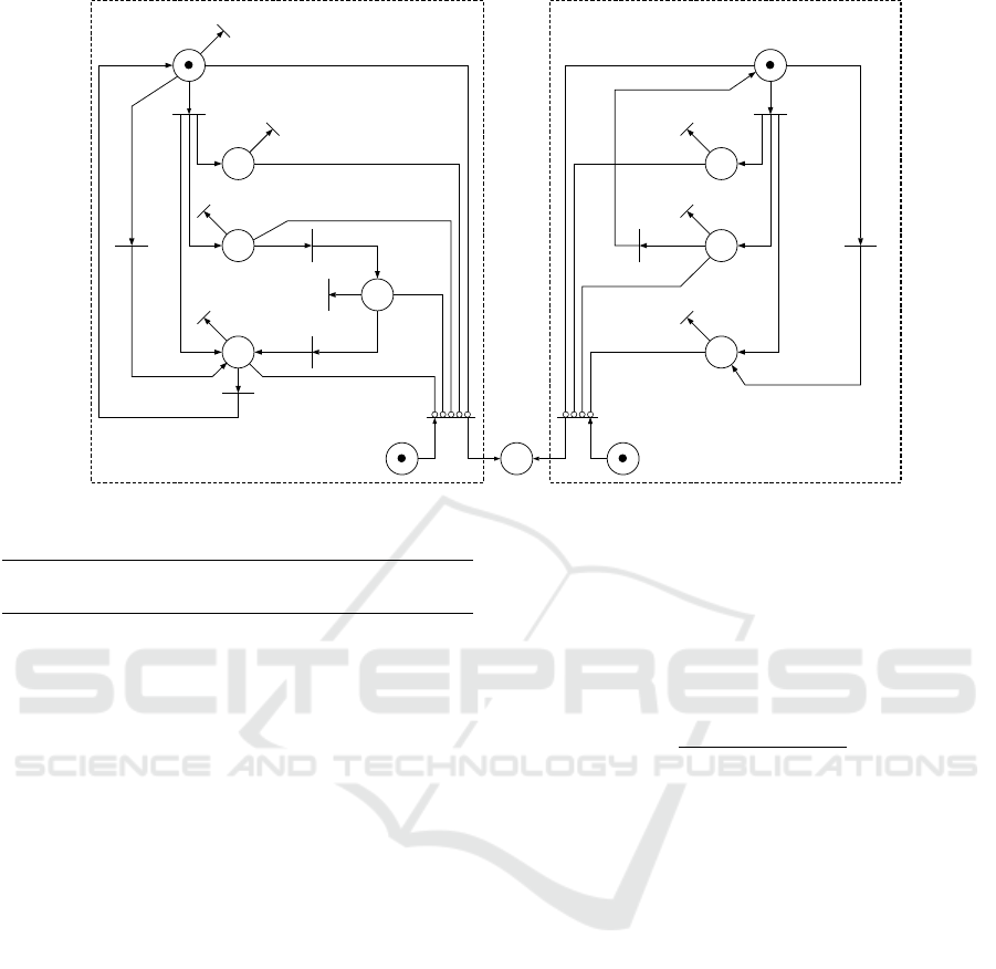
Example 2. Consider again the modular system G =
G
1
kG
2
, where G
1
and G
2
are shown in Figure 1. Al-
though, as pointed out in Example 1, L is not syn-
chronously diagnosable, let us construct the SPND
for this example. Following the method presented in
(Cabral et al., 2015a; Cabral and Moreira, 2017), the
SPND depicted in Figure 7 is obtained. Notice that if
the system generates the failure trace hσ
f
eh(eh)
?
, the
failure event σ
f
is not diagnosed since none of the
Petri nets N
D
1
or N
D
2
loses all their tokens.
When the system generates the failure trace
hσ
f
eh(eh)
?
, as a consequence of the occurrence of
event h, observable transition t
2,1
of Petri net N
D
2
fires, removing a token from place 0N
2
and adding
a token to places 1N
2
, 2N
2
, and 3N
2
. Then, when
event e is observed, transition t
1,2
of N
D
1
and tran-
sition t
2,4
of N
D
2
fire, removing a token from places
0N
1
and 2N
2
, and adding a token to places 3N
1
and
0N
2
. However, transition ((0, 2, N),e,(3, 0,N)) does
not exist in automaton G
N
, as shown in Figure 2, and
therefore, the simultaneous firing of transitions t
1,2
and t
2,4
should be avoided. Indeed, it can be seen in
Figure 2 that event e is feasible only in states (0,0, N)
or (3,2, N) of G
N
, i.e., if the system is in state 0 in au-
tomaton G
1
and state 0 in automaton G
2
, or in state 3
in automaton G
1
and state 2 in automaton G
2
. Thus,
if we add a condition to the firing of transition t
1,2
, as-
sociated with the marking of place 0N
2
of N
D
2
, and a
condition to the firing of t
2,4
associated with the mark-
ing of place 3N
1
of N
D
1
, the simultaneous firing of t
1,2
and t
2,4
would be avoided.
In the following section, we propose a modifica-
tion of the SPND in order to decrease the estimated
normal observed language for synchronous diagnosis.
3 CONDITIONAL
SYNCHRONIZED PETRI NET
DIAGNOSER
In this paper, we propose a modification in the SPND,
in order to allow an observable transition to fire in
a state observer Petri net only if this transition also
exists in the normal automaton of the system G
N
,
leading to the conditional synchronized Petri net di-
agnoser (CSPND) N
D,c
. In order to do so, we add
conditions to the observable transitions of the Petri
net state observers N
SO
k
, for k = 1, . .. ,r, based on
G
N
. These conditions are boolean expressions associ-
ated with places of the Petri net state observers N
SO
j
,
for j = 1, . . . ,r, and j 6= k.
As illustrated in Example 2, the addition of con-
ditions to the observable transitions of N
SO
k
based
on the normal automaton model G
N
can contribute
to the diagnosis of the failure event. This leads to
conditional Petri net state observers N
c
SO
k
, where
each transition is labeled with observable events and
conditions that depend on the marking of places of
Petri nets N
c
SO
j
, for j = 1, . . ., r, j 6= k. These condi-
tions are selected based on the possible observable
transitions of G
N
. Thus, Petri net N
c
SO
k
is an eight-
tuple N
c
SO
k
= (P
SO
k
,T
c
SO
k
,Pre
c
SO
k
,Post
c
SO
k
,x
0,SO
k
,
Σ
k,o
,C
SO
k
,l
c
SO
k
), where l
c
SO
k
: T
c
SO
k
→ 2
Σ
k,o
×C
SO
k
is a
labeling function that associates to each transition in
T
c
SO
k
a set of events from 2
Σ
k,o
and a condition C from
C
SO
k
, associated with the places of Petri nets N
c
SO
j
,
for j = 1, . . . ,r, j 6= k.
In the sequel, we present Algorithm 1 for the com-
putation of the conditional synchronized Petri net di-
agnoser N
D,c
.
Conditional Synchronized Diagnoser for Modular Discrete-event Systems
93
N
D
1
N
D
2
0N
1
c, g
1N
1
a, c, g, e
2N
1
3N
1
4N
1
e
t
1,2
t
1,1
a
t
1,4
c
t
1,5
a, g, e
t
1,6
g
t
1,7
a, c, e
t
1,8
a, c, g
t
1,10
e
t
1,9
t
f
1
0N
2
t
2,1
h
1N
2
h, e
t
2,3
2N
2
e
t
2,4
3N
2
h, e
t
2,6
e
t
2,2
P
N
2
t
f
2
P
N
1
P
F
h
t
2,5
t
1,3
Figure 7: Synchronized Petri net diagnoser of Example 2.
Algorithm 1. Conditional synchronized Petri net di-
agnoser N
D,c
.
Input: Petri net state observers N
SO
k
= (P
SO
k
,T
SO
k
,
Pre
SO
k
,Post
SO
k
,x
0,SO
k
,Σ
k,o
,l
SO
k
), for k = 1, . .. , r, and
automaton G
N
.
Output: Conditional synchronized Petri net diag-
noser N
D,c
.
1: Compute the conditional state observer Petri
nets N
c
SO
k
= (P
SO
k
,T
c
SO
k
,Pre
c
SO
k
,Post
c
SO
k
,x
0,SO
k
,
Σ
k,o
,C
SO
k
,l
c
SO
k
), as follows:
1.1: Let T
c
0
SO
k
=
/
0. Create a new transition
t
c
k
for each transition ˜q
N
k
= f
N
k
(q
N
k
,σ) de-
fined in G
N
k
, where ˜q
N
k
,q
N
k
∈ Q
N
k
, and
σ ∈ Σ
k,o
. For each transition t
c
k
, define
Pre
c
SO
k
(p
k
,t
c
k
) = 1, if p
k
corresponds to state
q
N
k
, and Pre
c
SO
k
(p
k
,t
c
k
) = 0, otherwise, and do
T
c
0
SO
k
= T
c
0
SO
k
∪ {t
c
k
}.
1.2: Define T
c
SO
k
= T
SO
k
∪ T
c
0
SO
k
.
1.3: Define Pre
c
SO
k
: P
SO
k
× T
c
SO
k
→ N and
Post
c
SO
k
: T
c
SO
k
× P
SO
k
→ N such that
Pre
c
SO
k
(p
k
,t
k
) = Pre
SO
k
(p
k
,t
k
), and
Post
c
SO
k
(t
k
, p
k
) = Post
SO
k
(t
k
, p
k
) for
all p
k
∈ P
SO
k
and t
k
∈ T
SO
k
, and
Post
c
SO
k
(t
c
k
, p
k
) = Post
c
SO
k
(t
c
k
, p
k
) = 0, for
all t
c
k
∈ T
c
0
SO
k
and p
k
∈ P
SO
k
.
1.4: Define l
c
SO
k
: T
c
SO
k
→ 2
Σ
k,o
×C
SO
k
as:
l
c
SO
k
(t
k,i
)=
(l
SO
k
(t
k,i
),C
k,i
), if t
k,i
∈T
k,o
∪ T
c
0
SO
k
(l
SO
k
(t
k,i
),1), otherwise,
(4)
with
C
k,i
=
(
[
V
r
j=1, j6=k
(
W
`
p
j,`
)], if t
k,i
∈ T
k,o
[
V
r
j=1, j6=k
(
W
`
p
j,`
)], if t
k,i
∈ T
c
0
SO
k
(5)
for all places p
j,`
∈ P
SO
j
such that I(t
k,i
) and
p
j,`
correspond to states in Q
N
k
and Q
N
j
that
are the k-th and j-th coordinates of a state q
N
∈
Q
N
, respectively, where f
N
(q
N
,σ) is defined for
σ ∈ l
SO
k
(t
k,i
).
1.5: Define the initial marking of N
c
SO
k
as x
c
0,SO
k
=
x
0,SO
k
, for k = 1, .. ., r.
2: Compute the Petri net N
c
D
k
= (P
c
D
k
,T
c
D
k
,
Pre
c
D
k
,Post
c
D
k
,In
c
D
k
,x
c
0,D
k
,Σ
k,o
,C
SO
k
,l
c
SO
k
), where
In
c
D
k
: P
c
D
k
× T
c
D
k
→ {0,1} denotes the function of
inhibitor arcs, as follows:
2.1: Add to N
c
SO
k
a transition t
f
k
labeled with the
always occurring event λ. Define T
c
D
k
= T
SO
k
∪
{t
f
k
}.
2.2: Add to N
c
SO
k
a place p
N
k
, and define
Pre
c
D
k
(p
N
k
,t
f
k
) = 1. Set x
c
0,D
k
(p
N
k
) = 1, and de-
fine P
c
D
k
= P
SO
k
∪ {p
N
k
}.
2.3: Define In
c
D
k
(p
c
D
k
,t
f
k
) = 1 and In
D
k
(p
c
D
k
,t
c
SO
k
) =
0, ∀p
c
D
k
∈ P
c
D
k
and ∀t
c
SO
k
∈ T
c
SO
k
.
3: Compute the conditional synchronized Petri
net diagnoser N
D,c
= (P
c
D
,T
c
D
,Pre
c
D
,Post
c
D
,
ICINCO 2017 - 14th International Conference on Informatics in Control, Automation and Robotics
94

In
c
D
,x
c
0,D
,Σ
o
,C
c
D
,l
c
D
), as follows:
3.1: Form a unique Petri net by grouping all Petri
nets N
c
D
k
, for k = 1, .. . ,r.
3.2: Add a place p
F
and define Post
c
D
(t
f
k
, p
F
) = 1,
for k = 1, .. ., r. Set x
c
0,D
(p
F
) = 0.
In the following, we present an example of the
CSPND N
D,c
for the modular system G of Example
1.
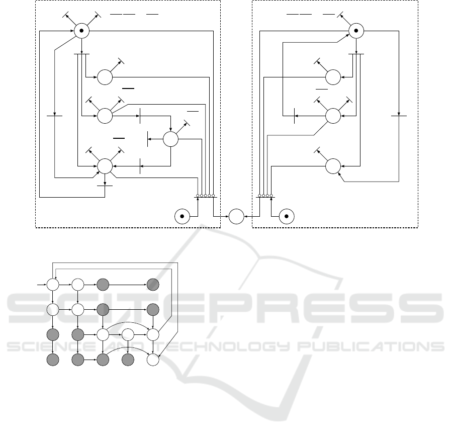
Example 3. Consider the modular system G =
G
1
kG
2
, where G
1
and G
2
are depicted in Figure 1.
Following the steps of Algorithm 1, the conditional
synchronized Petri net diagnoser N
D,c
, shown in Fig-
ure 8, is constructed. Notice that, if the system gen-
erates the failure trace hσ
f
eh(eh)
?
, the failure event
σ
f
is diagnosed by the CSPND N
D,c
after the first ob-
servation of event e, since both Petri nets N
D,c
1
and
N
D,c
2
lose all tokens.
It is important to notice that the conditions added
to N
D
prevent observable transitions that cannot occur
in G
N
to be considered as belonging to the estimated
normal observed behavior of the system. The practi-
cal consequence of this fact is a decrease in the ob-
served augmented normal language for synchronous
diagnosis P
o
(L
N
a
), leading to an observed condi-
tional augmented normal language P
o
(L
N
a,c
), where
P
o
(L
N
a,c
) ⊆ P
o
(L
N
a
). Moreover, since the observed
language of automaton G
R
N
is equivalent to P
o
(L
N
a
),
in order to model the language P
o
(L
N
a,c
), we have to
erase the observable transitions of G
R
N
according to
G
N
, leading to the conditional normal behavior model
automaton G
R
N
c
. This can be done by following the
steps of the algorithm presented in the sequel.
Algorithm 2. Conditional normal behavior model
Input: Automata G
N
and G
R
N
.
Output: Automaton G
R
N
c
.
1: Flag the transitions f
R
N
(q
R
N
,σ) = q
R
N
0
, such that
[(q
R
N
6∈ Q
N
) ∨ (q
R
N
0
6∈ Q
N
)] ∧ (σ ∈ Σ
o
) of G
R
N
.
2: Compute G
R
N
0
by eliminating the flagged transi-
tions from G
R
N
.
3: Compute G
R
N
c
= Ac(G
R
N
0
).
In the following, we present a theorem that en-
sures that the removal of observable transitions from
G
R
N
by Algorithm 2 in order to compute G
R
N
c
has the
same effect as the conditions added to N
D
in order to
obtain N
D,c
.
Theorem 1. Consider automaton G
R
N
c
obtained by
following the steps of Algorithm 2. The observed lan-
guage of G
R
N
c
, P
R
o
(L(G
R
N
c
)) = P
o
(L
N
a,c
), corresponds
to the conditional augmented normal language.
Proof. In order to prove Theorem 1, we must show
that the conditions added to the SPND N
D
have the
same effect as erasing the observable transitions of
G
R
N
to compute automaton G
R
N
c
. Notice that the con-
ditions added to an observable transition in a Petri net
state observer N
SO
k
only allow this transition to fire if
a set of places of the other Petri nets have tokens as-
signed. This set of places correspond to a set of states
of the normal behavior models of the components of
the system that form a state in G
N
, where this observ-
able event is active. Therefore, this transition can only
fire in the CSPND N
D,c
if there exists a correspondent
observable transition in G
N
.
Example 4. Consider automata G
N
and G
R
N
depicted
in Figures 2 and 6, respectively. Following the steps
of Algorithm 2, automaton G
R
N
c
, shown in Figure 9, is
computed. Notice that there are no observable tran-
sitions in G
R
N
c
that do not belong to G
N
. It is im-
portant to remark that the augmented normal trace
ω
a,1
= hσ
R
2
e(hσ
R
2
e)
?
, that belongs to G
R
N
, whose ob-
servation in Σ
o
is P
R
o
(ω
a,1
) = he(he)
?
was eliminated
and it is not possible to occur in G
R
N
c
. The trace ω
a,1
has the same observation in Σ
o
that the failure trace
st = hσ
f
e(he)
n
, which makes the system G not syn-
chronously diagnosable. However, after eliminating
the observable transitions of G
R
N
that do not belong
to G
N
, the normal augmented trace ω
a,1
is not possi-
ble to occur in G
R
N
c
, and the failure trace st becomes
conditionally synchronously diagnosable.
It is important to notice that, even with the elimi-
nation of the observable transitions from G
R
N
that do
not belong to G
N
, the observable normal language
for conditional synchronous diagnosis can still be a
larger set than the observable normal language of
the system, i.e., P
R
o
(G
R
N
c
) ⊇ P
o
(L
N
). In order to see
this fact, consider the normal augmented trace ω
a,2
=
haσ
u
R2
σ
u
R1
σ
u
R1
e(haσ
u
R2
σ
u
R1
σ
u
R1
e)
?
, whose observa-
tion in Σ
o
is P
R
o
(ω
a,2
) = hae(hae)
?
. Notice that
P
R
o
(ω
a,2
) does not belong to the observable nor-
mal language of the system P
o
(L
N
), P
R
o
(ω
a,2
) =
hae(hae)
?
6∈ P
o
(L
N
).
It is important to remark that the observed nor-
mal language for the conditional synchronous diag-
nosis P
o
(L
N
a,c
) is a superset of the observed normal
language of the composed system P
o
(L
N
). Therefore,
even if a modular system is diagnosable, this system
is not necessarily conditionally synchronously diag-
nosable. This leads to the following definition of con-
ditional synchronous diagnosability.
Definition 4. Let L and L
N
⊂ L denote the languages
generated by G and G
N
, respectively, and let L
F
=
L \ L
N
. Consider that the system is composed of r
modules, such that G
N
= k
r
k=1
G
N
k
, where G
N
k
is the
automaton that models the normal behavior of G
k
,
Conditional Synchronized Diagnoser for Modular Discrete-event Systems
95
N
c
D
1
N
c
D
2
0N
1
c, g
1N
1
a, c, g, e
2N
1
c.[
2N
2
]
3N
1
4N
1
e.[0N
2
]
t
1,3
t
1,11
t
1,2
t
1,1
a.[0N
2
, 1N
2
]
a.[
0N
2
.1N
2
], e.[0N
2
]
t
1,4
c.[2N
2
]
t
1,5
t
1,12
a, g, e
t
1,6
g.[2N
2
]
t
1,7
g.[
2N
2
]
t
1,13
a, c, e
t
1,8
e.[
2N
2
]
a, c, g
t
1,10
t
1,14
e.[2N
2
]
t
1,9
t
f
1
0N
2
h.[0N
1
.1N
1
], e.[0N
1
]
t
2,1
h.[0N
1
, 1N
1
]
1N
2
h, e
t
2,3
2N
2
h
t
2,8
t
2,5
e.[
3N
1
]
e.[3N
1
]
t
2,4
3N
2
h, e
t
2,6
t
2,7
e.[0N
1
]
t
2,2
P
N
2
t
f
2
P
N
1
P
F
Figure 8: Conditional synchronized Petri net diagnoser N
D,c
of Example 3.
0,0
a
hh
σ
u
R
2
1,0
0,1 1,1
σ
u
R
1
σ
u
R
1
σ
u
R
1
σ
u
R
1
0,2 1,2
σ
u
R
2
σ
u
R
2
σ
u
R
2
a
σ
u
R
1
σ
u
R
1
c
g
σ
u
R
2
σ
u
R
1
0,3 1,3
σ
u
R
2
σ
u
R
2
σ
u
R
2
σ
u
R
1
2,0
2,1
2,2
2,3
4,2
4,3
3,0
3,1
3,2
3,3
σ
u
R
2
e
e
Figure 9: Automaton G
R
N
c
of Example 4.
and let L
N
k
denote the language generated by G
N
k
,
for k = 1,. . . , r. Then, L is said to be condition-
ally synchronously diagnosable with respect to L
N
a,c
,
P
o
: Σ
?
→ Σ
?
o
, and Σ
f
if
(∃n ∈ N)(∀s ∈ L
F
)(∀st ∈ L
F
,ktk ≥ n) ⇒
(P
o
(st) 6∈ P
o
(L
N
a,c
)).
Notice that, according to Definition 4, in order to
verify if a system is conditionally synchronously di-
agnosable, it is necessary to verify if there is an arbi-
trarily long length failure trace with the same observa-
tion as a normal trace that belongs to P
o
(L
N
a,c
). Since,
as shown in Theorem 1, P
R
o
(L(G
R
N
c
)) = P
o
(L
N
a,c
), and
all unobservable events of G
R
N
c
are renamed, in order
to verify the conditional synchronous diagnosability
of a system, the algorithm proposed in (Cabral and
Moreira, 2017) for verifying synchronous diagnos-
ability can be used. In order to do so, instead of using
G
V
= G
R
N
kG
F
, it is necessary to build G
V,c
= G
R
N
c
kG
F
and search for cyclic paths formed with states labeled
with F and events there are not renamed. If there ex-
ists a cyclic path in G
V,c
with these characteristics,
then the system is not conditionally synchronously
diagnosable. It can be seen that for the running ex-
ample of this paper G
V,c
does not have cyclic paths
whose states are labeled with F and at least one event
belongs to Σ. Thus, L is conditionally synchronously
diagnosable.
Remark 1. It is important to remark that since
P
o
(L
N
a
) ⊇ P
o
(L
N
a
,c
), even if a system is synchronously
diagnosable, the delay bound for conditional syn-
chronous diagnosis can be smaller than for syn-
chronous diagnosis. In (Cabral and Moreira, 2017),
a method for the computation of the delay bound for
synchronous diagnosis that uses the verifier automa-
ton G
V
is proposed. The same method can be used for
the computation of the delay bound for conditional
synchronous diagnosis by using the verifier automa-
ton G
V,c
instead of G
V
.
4 CONCLUSIONS
In this paper, a conditional synchronized Petri net di-
agnoser is proposed. In order to do so, we propose
the addition of conditions to the observable transitions
of the synchronized Petri net diagnoser (SPND) pre-
sented in (Cabral et al., 2015a; Cabral and Moreira,
2017). We show that the conditional synchronous di-
agnosis can have a smaller delay bound than the syn-
chronous diagnosis approach. Moreover, systems that
ICINCO 2017 - 14th International Conference on Informatics in Control, Automation and Robotics
96

are not synchronously diagnosable can be condition-
ally synchronously diagnosable.
ACKNOWLEDGEMENTS
This paper was partially supported by the Brazilian
Research Council (CNPq) under grant 309084/2014-
8.
REFERENCES
Alayan, H. and Newcomb, R. W. (1987). Binary Petri-net
relationships. IEEE Transactions on Circuits and Sys-
tems, CAS-34:565–568.
Basilio, J. C., Lima, S. T. S., Lafortune, S., and Moreira,
M. V. (2012). Computation of minimal event bases
that ensure diagnosability. Discrete Event Dynamic
Systems: Theory And Applications, 22:249–292.
Cabasino, M. P., Giua, A., Paoli, A., and Seatzu, C. (2013).
Decentralized Diagnosis of Discrete Event Systems
using labeled Petri nets. IEEE Transactions on Sys-
tems, Man, and Cybernetics: Systems, 43(6):1477–
1485.
Cabasino, M. P., Giua, A., and Seatzu, C. (2010). Fault de-
tection for discrete event systems using Petri nets with
unobservable transitions. Automatica, 46():1531–
1539.
Cabral, F. G. and Moreira, M. V. (2017). Online failure di-
agnosis of modular discrete-event systems. Automatic
Control, IEEE Transactions on. Submitted for publi-
cation.
Cabral, F. G., Moreira, M. V., and Diene, O. (2015a). Online
fault diagnosis of modular discrete-event systems. In
Decision and Control (CDC), 2015 IEEE 54th Annual
Conference on, pages 4450–4455. IEEE.
Cabral, F. G., Moreira, M. V., Diene, O., and Basilio, J. C.
(2015b). A Petri net diagnoser for discrete event sys-
tems modeled by finite state automata. IEEE Transac-
tions on Automatic Control, pages 59–71.
Carvalho, L. K., Basilio, J. C., and Moreira, M. V.
(2012). Robust diagnosis of discrete-event systems
against intermittent loss of observations. Automatica,
48(9):2068–2078.
Carvalho, L. K., Moreira, M. V., and Basilio, J. C. (2011).
Generalized robust diagnosability of discrete event
systems. In 18th IFAC World Congress, pages 8737–
8742, Milano, Italy.
Carvalho, L. K., Moreira, M. V., Basilio, J. C., and Lafor-
tune, S. (2013). Robust diagnosis of discrete-event
systems against permanent loss of observations. Au-
tomatica, 49(1):223–231.
Cassandras, C. and Lafortune, S. (2008). Introduction to
Discrete Event System. Springer-Verlag New York,
Inc., Secaucus, NJ.
Contant, O., Lafortune, S., and Teneketzis, D. (2006). Di-
agnosability of discrete event systems with modular
structure. Discrete Event Dynamic Systems: Theory
And Applications, 16(1):9–37.
Davi, R. and Alla, H. (2005). Discrete, Continuous and
Hybrid Petri Nets. Springer.
Debouk, R., Malik, R., and Brandin, B. (2002). A modular
architecture for diagnosis of discrete event systems. In
41st IEEE Conference on Decision and Control, pages
417–422, Las Vegas, Nevada USA.
Fanti, M. P., Mangini, A. M., and Ukovich, W. (2013). Fault
detection by labeled petri nets in centralized and dis-
tributed approaches. Automation Science and Engi-
neering, IEEE Transactions on, 10(2):392–404.
Garc
´
ıa, E., Correcher, A., Morant, F., Quiles, E., and
Blasco-Gim
´
enez, R. (2006). Centralized modular di-
agnosis and the phenomenon of coupling. Discrete
Event Dynamic Systems, 16(3):311–326.
Kan John, P., Grastien, A., and Pencol
´
e, Y. (2010). Synthe-
sis of a distributed and accurate diagnoser. In 21st In-
ternational Workshop on Principles of Diagnosis (DX-
10), pages 209–216.
Moreira, M. V., Jesus, T. C., and Basilio, J. C. (2011). Poly-
nomial time verification of decentralized diagnosabil-
ity of discrete event systems. IEEE Transactions on
Automatic Control, pages 1679–1684.
Qiu, W. and Kumar, R. (2006). Decentralized failure diag-
nosis of discrete event systems. IEEE Transactions on
Systems, Man, and Cybernetics Part A:Systems and
Humans, 36(2):384–395.
Sampath, M., Sengupta, R., Lafortune, S., Sinnamohideen,
K., and Teneketzis, D. (1995). Diagnosability of
discrete-event systems. IEEE Trans. on Automatic
Control, 40(9):1555–1575.
Sampath, M., Sengupta, R., Lafortune, S., Sinnamohideen,
K., and Teneketzis, D. (1996). Failure diagnosis using
discrete-event models. IEEE Trans. on Control Sys-
tems Technology, 4(2):105–124.
Santoro, L. P. M., Moreira, M. V., and Basilio, J. C. (2017).
Computation of minimal diagnosis bases of discrete-
event systems using verifiers. Automatica, 77:93–102.
Schmidt, K. W. (2013). Verification of modular diagnos-
ability with local specifications for discrete-event sys-
tems. IEEE Transactions on Systems, Man, and Cy-
bernetics: Systems, 43(5):1130–1140.
Tomola, J. H. A., Cabral, F. G., Carvalho, L. K.,
and Moreira, M. V. (2016). Robust disjunctive-
codiagnosability of discrete-event systems
against permanent loss of observations. IEEE
Transactions on Automatic Control. DOI:
10.1109/TAC.2016.2638042.
Zaytoon, J. and Lafortune, S. (2013). Overview of fault
diagnosis methods for discrete event systems. Annual
Reviews in Control, 37(2):308–320.
Zhou, C., Kumar, R., and Sreenivas, R. S. (2008). De-
centralized modular diagnosis of concurrent discrete
event systems. In 9th Workshop on Discrete Event
Systems, pages 388–393, G
¨
oteborg, Sweden.
Conditional Synchronized Diagnoser for Modular Discrete-event Systems
97
