Quadrotor Attitude Control using

Incremental Nonlinear Dynamics Inversion

Rodrigo Coelho

, Alexandra Moutinho

and Jos

e Raul Azinheira

Instituto Superior T

ecnico, Universidade de Lisboa, Portugal

IDMEC, Instituto Superior T

ecnico, Universidade de Lisboa, Portugal

Keywords:

Incremental Nonlinear Dynamics Inversion, Quadrotor, Attitude Control, Sensor-based Control.

Abstract:

Given the large ﬂight envelope of vertical take-off and landing vehicles, and the nonlinear nature of multi-

rotor aircraft, especially in aggressive maneuvering, nonlinear control strategies are often considered. Yet,

most available solutions are model dependent and thus require a precise knowledge of the system dynamics,

including the hard to model aerodynamics. This paper proposes a sensor-based approach to the problem. It

considers a recent strategy based on incremental control and Nonlinear Dynamics Inversion (NDI), the Incre-

mental Nonlinear Dynamics Inversion (INDI), to solve the attitude control problem of quadrotors. The INDI

general formulation is presented, and then applied considering the attitude stabilization of a quadrotor. In

order to apply the INDI solution to this case study, a linear predictor for the angular acceleration is provided.

Simulation results demonstrate the robustness of this sensor-based approach to model-parameter uncertainties

and wind disturbances. An analysis is also done regarding the tuning of INDI parameters and its sensitivity to

the chosen sampling time.

1 INTRODUCTION

In these past few decades there has been a growing

interest in unmanned aerial vehicles (UAVs). These

vehicles are characterized by the absence of an on-

board human pilot, being instead controlled remotely

and/or by an onboard control system. This interest is

brought by the recent technological advances in the

area of microprocessors, microcontrollers and sensor

systems as well as their respective manufacturing pro-

cesses. Thanks to these advances the prices and sizes

have been continuously decreasing and consequently

UAVs have also become cheaper, smaller and easier to

build. Their applications were initially reserved to the

domain of military operations, where they decrease

the risk of human loss and can increase efﬁciency,

especially in tedious and/or dangerous missions such

as covert or surveillance operations. Now UAVs are

open to the general public and are being applied to

new and different domains every day, such as aerial

footage, ﬁre prevention, search and rescue operations,

monitoring of agriculture crops, infrastructure inspec-

tion and even multimedia or pure recreation.

There is a special interest in aircrafts with Verti-

cal Take-Off and Landing (VTOL) capabilities due to

their ability to operate with tighter spatial constraints

than traditional ﬁxed-wing aircraft. In this category

the most studied aircraft are the helicopters and the

multirotors where we have a need for robust and sta-

ble control as there is absence of dynamic pressure

that in conventional aircraft is brought by the for-

ward ﬂight speed, ruling out inherent stability. Due to

the unstable and nonlinear nature of multirotors and

the large ﬂight envelope associated to a VTOL, espe-

cially if aggressive maneuvering is necessary, nonlin-

ear control strategies must be considered.

Several nonlinear solutions are presented for this

problem such as Gain-Scheduling (Sadeghzadeh

et al., 2011), Nonlinear Dynamics Inversion

(NDI) (Mallikarjunan and et al., 2012), and Back-

stepping (Mallikarjunan and et al., 2012), as well

as adaptive (Krstic et al., 1995; Sadeghzadeh et al.,

2011; Mallikarjunan and et al., 2012; Bastin, 2013)

and robust (Liao et al., 2002; Goman and Kolesnikov,

1998) control techniques. However, these are ap-

proaches based on the knowledge of the system,

and as such called model-based solutions. For the

particular case of aircraft control, this model require-

ment can prove to be costly and time-consuming, as

the aerodynamic coefﬁcients, for example, require

extensive wind-tunnel or ﬂight tests to be properly

identiﬁed.

Coelho, R., Moutinho, A. and Azinheira, J.

Quadrotor Attitude Control using Incremental Nonlinear Dynamics Inversion.

DOI: 10.5220/0006435900980109

In Proceedings of the 14th International Conference on Informatics in Control, Automation and Robotics (ICINCO 2017) - Volume 2, pages 98-109

ISBN: Not Available

Due to the general development of micro-electro-

mechanical systems (MEMS), smaller, more accu-

rate and more accessible sensors are available. This

allows for sensor-based control approaches, where

model knowledge is replaced by variable measure-

ments. An example of these approaches is the In-

cremental Nonlinear Dynamics Inversion (INDI), an

incremental variation of the Nonlinear Dynamics In-

version, and object of some recent studies regarding

ﬂight control (Sieberling et al., 2010; Simpl

ıcio et al.,

2013). It is relatively easy to design as it does not

need the complete system model, only the input re-

lated part, because it uses sensor measurements to

compensate for the state-only dependent dynamics

such as the hard to model aerodynamics. This makes

it more robust than traditional feedback linearization

or NDI as it is not so sensitive to modeling errors. The

downside are stricter requirements in the sampling

frequency and the need for accurate sensors reading

and/or variables estimation.

This paper addresses the INDI solution for the

quadrotor attitude control problem. In order to better

understand and evaluate this approach, the results pre-

sented test its robustness to model uncertainties and

wind disturbances, as well as provide an insight on its

sensitivity to design parameters.

The remaining of this paper is organized as fol-

lows. After the general formulation of INDI is intro-

duced (sec. 2), and the model of the quadrotor is de-

ﬁned (sec. 3), the INDI control approach is applied to

the quadrotor attitude control problem (sec. 4). Like

for other feedback linearization approaches, this cor-

responds to the usual two-steps procedure of lineariz-

ing the system (here using INDI) and then applying

linear control to the linearized system. The imple-

mentation requires that angular accelerations be avail-

able. In this paper they are estimated using a linear

predictor. In section 5, a parameter tuning study re-

garding the INDI controller and the linear estimator

is presented, followed by some simulation results that

illustrate the solution performance and its robustness

to model uncertainties and wind disturbances, as well

as its sensitivity to the sampling time. Finally, sec-

tion 7 closes with some ﬁnal remarks.

2 NONLINEAR DYNAMICS

INVERSION CONTROL

THEORY

In order to better understand the incremental ver-

sion of the nonlinear dynamics inversion, this section

presents both classic and incremental formulations of

this approach.

2.1 Nonlinear Dynamics Inversion

For the NDI formulation (Sieberling et al., 2010),

consider the following afﬁne n-th order MIMO sys-

tem

x = f(x) +G(x)u (1)

y = h(x) (2)

where x ∈ R

is the system state vector, u ∈ R

is the

input vector, f ∈ R

and h ∈ R

are smooth vector

ﬁelds, and G ∈ R

m×n

is a matrix with each column

∈ R

a smooth vector ﬁeld.

By differentiating (2) with respect to time we have

y =

dh(x)

∂h

∂x

x (3)

∂h

∂x

f(x) +

∂h

∂x

G(x)u (4)

= L

h(x) + L

h(x)u (5)

where L

h(x) and L

h(x) are the respective Lie

Derivatives of h(x) with respect to f and G. Assum-

ing L

h(x) is invertible, the control action u may be

isolated as:

u = (L

h(x))

−1

(

y − L

h(x)) (6)

For y = x and

y a desired system dynamics

, we

have L

h(x) = G(x) and L

h(x) = f(x) and we can

rewrite (6) as

u = (G(x))

−1

(

− f(x)) (7)

This produces a linearized system in the form

x =

2.2 Incremental Nonlinear Dynamics

Inversion

Opposed to NDI, INDI has no requirements for the

input dynamics, so we can use a more generic formu-

lation (Azinheira et al., 2015) for nonlinear systems

such as

x = f(x, u) (8)

If we linearize (8) around the previous time step con-

dition (x

) with t

= t − T

and T

being the con-

troller sampling time, we have

∼

∂f

∂x

(x − x

) +

∂f

∂u

(u − u

) (9)

where

= f(x

). Assuming a small enough sam-

pling time T

, the state variation between samples can

be considered negligible (x ≈ x

). We can then sim-

plify (9) as

x ≈

∂f

∂u

(u − u

) (10)

Quadrotor Attitude Control using Incremental Nonlinear Dynamics Inversion

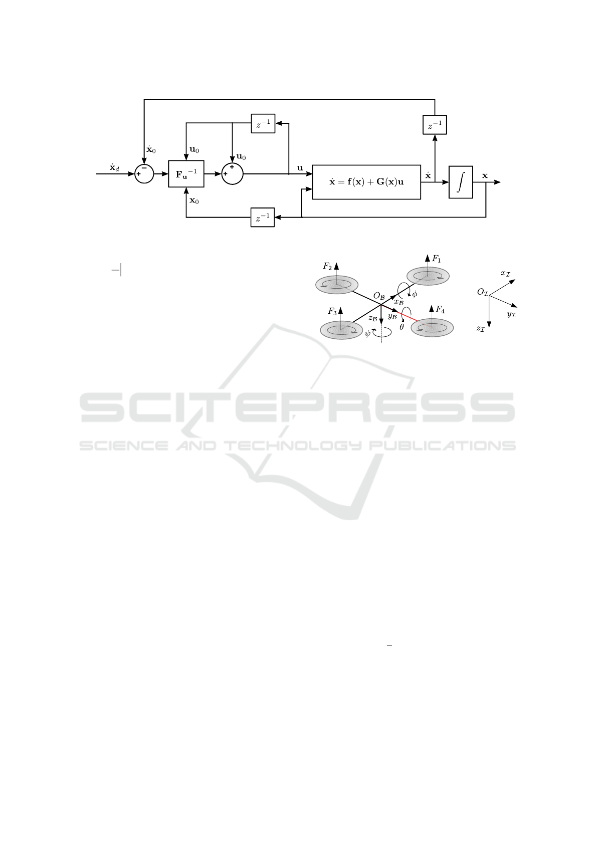
Figure 1: Block diagram representation of INDI control scheme.

Setting the desired dynamics as

x =

and deﬁn-

ing F

∂f

∂u

we obtain the following control input

u = u

+ F

−1

(

−

) (11)

where F

must be invertible and

, x

and u

must

be available.

The INDI control scheme is described by the

block diagram of ﬁgure 1.

3 QUADROTOR MODEL

This section presents the quadrotor nonlinear model.

In order to do so, the required reference frames are

ﬁrst introduced, followed by the kinematic and dy-

namic equations of motion.

3.1 Reference Frames

The ﬁrst spatial reference necessary is the inertial

frame, a frame that describes time and space homo-

geneously, isotropically, and in a time-independent

manner. We assume the ”ﬂat Earth” model and use

a North-East-Down (NED) frame located in the sur-

face of the Earth and centered on the quadrotor ini-

tial position, I = (O

), as the inertial ref-

erence frame. We will also deﬁne a frame ﬁxed to

the quadrotor and centered in its center of gravity,

B = (O

), as seen in ﬁgure 2.

Another frame that needs to be deﬁned is the In-

ertial Measurement Unit (IMU) frame. This frame is

centered in the IMU at d

IMU

= (x

IMU

) rel-

ative to the B frame and also ﬁxed to the quadrotor.

3.2 Kinematics

The kinematics describes the movement of the

quadrotor in the inertial frame I . To describe the po-

sition P of the quadrotor in I frame we can consider

Figure 2: Inertial and body-centered coordinate sys-

tems (Esteves et al., 2015).

the following transformation

P = R

V (12)

where P = (x, y,z)

is the body position in I frame,

V = (u,v,w)

is the linear velocity in B frame and R

is the rotation matrix from I to B frames expressed

using the quadrotor attitude represented using quater-

nions Q = (q

)

R =





1 − 2q

− 2q

2(q

+ q

) 2(q

− q

)

2(q

− q

) 1 − 2q

− 2q

2(q

+ q

)

2(q

+ q

) 2(q

− q

) 1 − 2q

− 2q





(13)

The rotational kinematics is described by

Q = S

ω (14)

where ω = (p,q,r)

is the angular velocity of the

quadrotor in the three main directions of B frame and

is a transformation matrix that using the quater-

nions attitude representation is deﬁned as

= −







−q







(15)

3.3 Dynamics

The dynamics model used is based on Newton-Euler

approach following (Stevens and Lewis, 2003).

ICINCO 2017 - 14th International Conference on Informatics in Control, Automation and Robotics

100

The translational dynamics is given by

V = F

+ F

+ mRg − mΩ

Ω

ΩV (16)

with F

= (0,0,

∑

j=1

)

the generalized rotors force

where F

, j = 1,2,3,4 is the force produced by rotor

j, F

∈ R

the aerodynamics drag force and mRg =

∈ R

the gravitational force expressed in B frame.

The cross-product matrix Ω

Ω

Ω = ω

ω× ∈ R

3×3

associated

with the Coriols term mΩ

Ω

ΩV is deﬁned as

Ω

Ω =





0 −r q

r 0 −p

−q p 0





(17)

The rotational dynamics is described by

ω = −Ω

Ω

ΩJω

ω + τ

(18)

with Ω

Ω

ΩJω

ω the Coriolis torque related term, τ



− F

), r

− F

∑

j=1

(−1)

j+1



the ro-

tors generalized torque where F

,τ

, j = 1, 2,3, 4 are

the force and torque produced by rotor j, r

is the

distance between the rotors and the quadrotor cen-

ter of mass, and where the aerodynamic drag torque

∈ R

was neglected given the quadrotor reduced

dimensions.

4 APPLICATION TO

QUADROTOR ATTITUDE

CONTROL

This section concerns the INDI application to the

quadrotor attitude control. Being a feedback lin-

earization methodology, the control design corre-

sponds to the usual two-steps procedure of lineariz-

ing the system (here using NDI or INDI for compari-

son) and then applying linear control to the linearized

system. The implementation also requires that angu-

lar accelerations be available, and with that purpose a

linear predictor is introduced. The complete solution

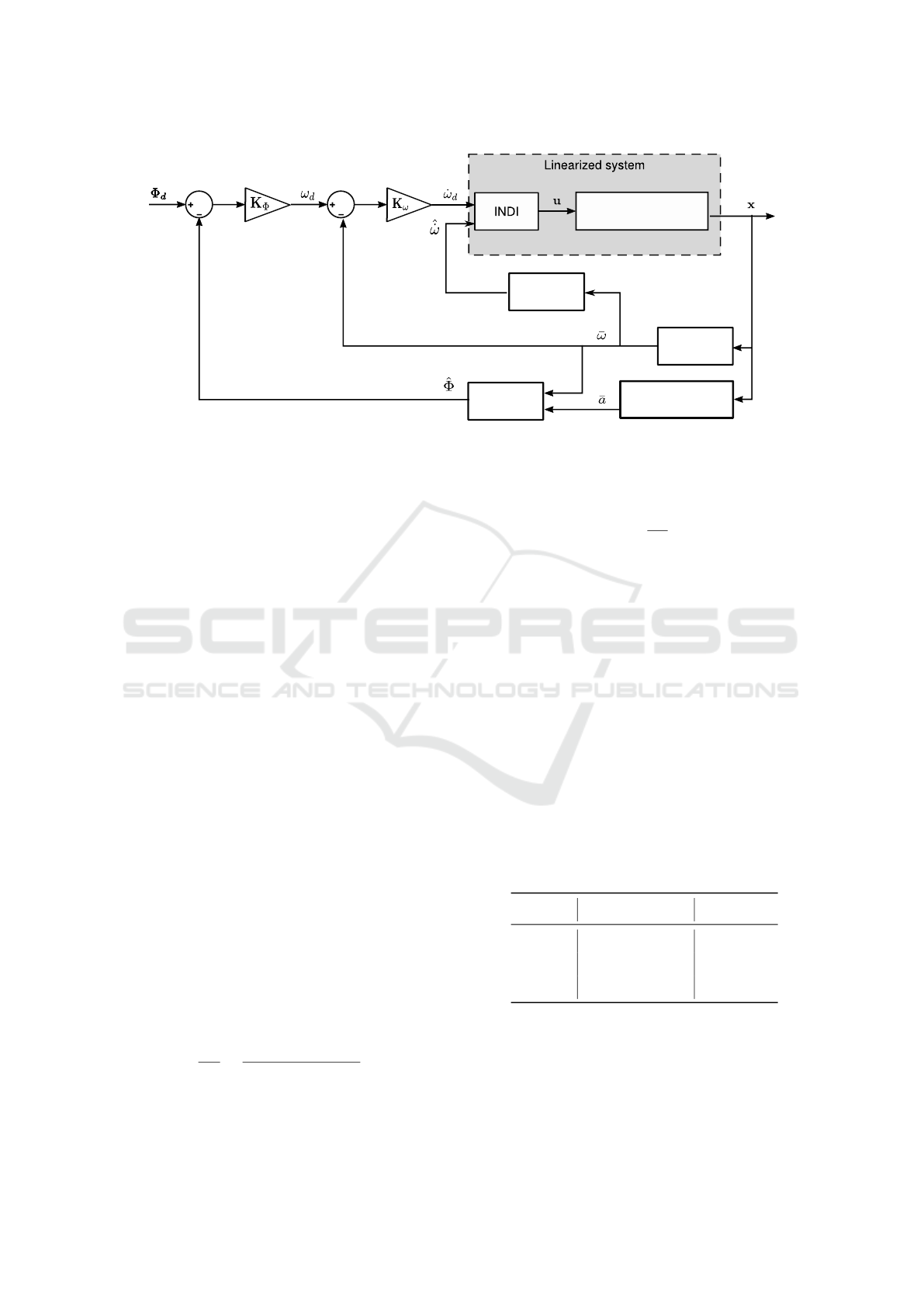
is depicted in the block diagram of ﬁg. 3.

4.1 System Linearization

In order to provide a better comparison between clas-

sic and incremental nonlinear dynamics inversion ap-

proaches, both formulations will be applied to the

quadrotor attitude control problem. Both formula-

tions consider x = [ω

, Q

]

, u = τ

and y = x.

4.1.1 NDI

For NDI we deﬁne f(x) and G(x) as

f(x) =



−J

−1

Ω

ΩJω



(19)

G(x) =



−1

4×3



(20)

Substituting (19)-(20) into (7) we obtain

u =



−1

4×3







−



−J

−1

Ω

ΩJω



(21)

where [·]

corresponds to the pseudo-inverse opera-

tion, and which simpliﬁed results in the NDI control

law

u = J(

+ J

−1

Ω

ΩJω

ω) (22)

where

∈ R

is a desired angular rate dynamics (ac-

celeration).

4.1.2 INDI

For INDI we deﬁne f(x,u) as

f(x,u) =



−J

−1

Ω

ΩJω

ω + J

−1



(23)

and the derivative

∂f

∂u



−1

4×3



(24)

Subsituting (23)-(24) into (11) we obtain

u = u



−1

4×3







−





(25)

that simpliﬁes into the INDI control law

u = u

+ J(

−

) (26)

where

∈ R

and

∈ R

are respectively desired

angular rate and attitude dynamics and

∈ R

and

∈ R

the last observed values of these variables.

Since this paper only addresses the attitude con-

trol, the vertical control is assumed to be dealt with

by another control loop, which deﬁnes the value of

the generalized forces F

= (0,0,

∑

j=1

)

, with F

the thrust force produced by rotor j, and therefore the

necessary thrust to keep the quadrotor hovering.

The control action deﬁned by the NDI or INDI

controllers corresponds to the generalized moments

applied to the quadrotor by the four rotors, u = τ

. In

order to apply the required control action, these gener-

alized moments need to be converted into the four ro-

tors angular speeds ω

. This transformation is called

control allocation and corresponds in this case to

u (27)

Quadrotor Attitude Control using Incremental Nonlinear Dynamics Inversion

101

Linear

predictor

Attitude

estimator

Rate gyro

Accelerometer

Quadrotor

Figure 3: Block diagram representation of proposed attitude control solution.

where ω

= (ω

,ω

)

are the rotors always

positive angular speed and





0 r

0 −r

−K





(28)

with K

, i = 1, 2,3, 4 the rotors torque coefﬁcients.

4.2 Linear Control

Applying the NDI and INDI to the quadrotor model

solves the problem of compensating the nonlineari-

ties in the system. It does not, however, solve the

complete attitude control problem. After the system

linearization done by INDI (or NDI), we may now use

linear control to stabilize each system state separately.

We will use the principle of time scale separation to

control the quadrotor attitude in two loops: an inner

one that stabilizes the attitude rate ω

ω and an outer loop

to control the attitude Φ

Φ itself.

For each loop we consider a simple proportional

controller

= K

(ω

− ω

ω) (29)

= K

(Φ

− Φ

Φ) (30)

where the gains K

∈ R

3×3

and K

∈ R

3×3

are diag-

onal matrices.

With the INDI linearization of the quadrotor dy-

namics, followed by the cascaded linear control, the

closed-loop system can be represented as a second

degree linear time-invariant system for each angle

, i = 1, 2,3 as

+ K

s + K

(31)

where K

and K

can be chosen according to our tar-

get damping coefﬁcient ξ

and natural frequency ω

= 2ξ

(32)

2ξ

(33)

These two parameters need to be chosen so that the

controlled system follows the performance require-

ments. We follow (Esteves et al., 2015) and choose

the following performance requirements for the atti-

tude response

• A 4.3% overshoot allowed;

• For roll and pitch, a rising time inferior to 1 sec-

ond and a settling time inferior to 3 seconds for a

step reference;

• For yaw, a rising time inferior to 4 sec and a set-

tling time inferior to 8 seconds for a step refer-

ence.

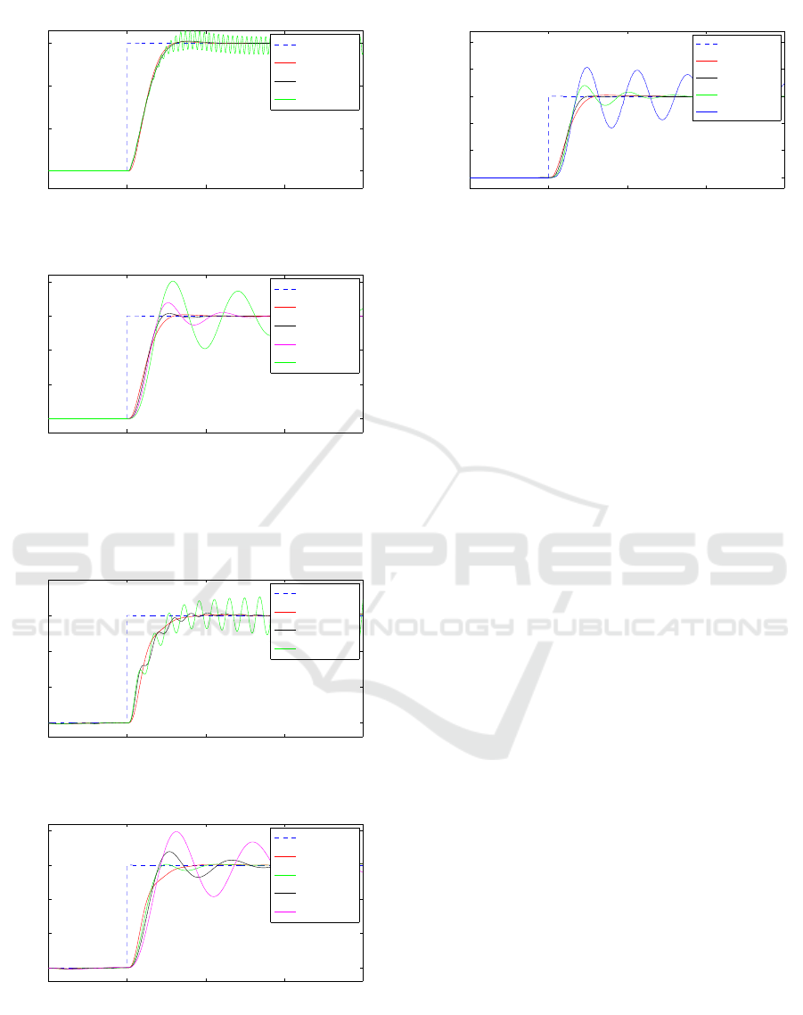
The parameters chosen are presented in table 1 and

the step response of the linearized system is presented

in ﬁgure 4.

Table 1: Linear controller gains.

Angle ξ ω

(rad/s) K

roll (φ) 0.79 6.32 10 4

pitch (θ) 0.79 6.32 10 4

yaw (ψ) 0.9 1.5 2.7 0.83

4.3 Linear Predictor for Angular

Acceleration Estimation

To implement the INDI controller, precise informa-

tion about the quadrotor angular acceleration

ω is

ICINCO 2017 - 14th International Conference on Informatics in Control, Automation and Robotics

102

Figure 4: Step response of the attitude closed-loop system.

needed. This information is not directly obtained

from sensor measurements, so an estimator is re-

quired. Following (Sieberling et al., 2010), we

present a linear predictor that takes advantage of the

INDI controller characteristics to solve the problem

of delay in real-world sensors. As the INDI controller

decouples the quadrotor dynamics and the linear con-

trol outer loops deﬁne each linearized state response,

we can design a decoupled linear estimator for each

state. The estimator structure is

∑

i=1

[θ

ω,i

k−i

+ θ

d,i

d,k−i

] + ε

ε (34)

with ω

d,k−i

the desired angular speed given by the

speed control loop, θ

ω,i

and θ

d,i

the measured and de-

sired angular speeds coefﬁcients, and ε

ε white noise.

To calculate the estimator coefﬁcients we use the

least-squares method with simulation data of a linear

system that represents the quadrotor behavior when

linearized with INDI and controlled by a decoupled

linear regulator. The SISO transfer function is

ω(s)

(s)

s + K

(35)

with ω(s) the angular speed, ω

(s) the desired angu-

lar speed, and K the gain imposed by the angular rate

inner control loop. The angular acceleration

ω is ob-

tained by differentiation.

With the knowledge of the angular rate ω

ω, the re-

spective reference ω

and the angular acceleration

ω,

the coefﬁcients θ

θ = [θ

] were estimated imple-

menting the least-squares method in Matlab

along

with a simulation of (35). The simulation run for 10 s

considering a pulse reference with a π/6 rad height

and 4 s duration, along with the system’s response for

the gains used in each angular rate control loop.

With the system’s response ω

ω and the angular ac-

celeration

ω calculated by numeric differentiation, we

solve

θ = (H

−1

z (36)

where H = [1 r

(t−1dt)

...r

(t−5dt)

(t−1dt)

...ω

(t−5dt)

]

is known as the design matrix that contains the refer-

ences r

and angular rates ω

in the last 5 samples and

z is the vector that contains the angular accelerations

one step ahead. Each row of matrix H and vector z

represent each sample taken from the simulation at a

frequency equal to the controller sampling frequency

1/T

5 SIMULATION RESULTS

This section presents the results and tests obtained

in a Matlab/Simulink

implementation. We ﬁrst ex-

plore the controller and estimator parameter tuning,

and after evaluate the overall approach performance,

namely its robustness to model uncertainties and its

sensitivity to sampling time.

5.1 Design Parameter Tuning

5.1.1 INDI Controller

Following (Azinheira et al., 2015), the INDI con-

troller implementation considers an additional control

parameter η. This parameter weights the update of the

control action ∆u = F

−1

(

−

) in relation to the last

input provided u

u = u

+ η∆u (37)

Taking into account the integrative characteristic of

INDI, we can compare η to an integral gain in a PID

controller. Whereas in a PID controller the integral

gain is meant to correct stationary errors, in INDI η is

meant to dampen the integration to help cope with the

imperfections in the actuation system and reduce the

error ampliﬁcation.

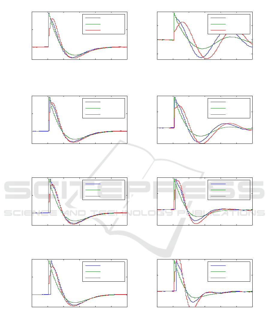
Figure 5 shows the required control action (angu-

lar speed for each motor ω

) and the respective re-

sponse of the system in roll angle φ to a step refer-

ence φ

= 15 deg for different values of the parameter

η. We can see for the case of η = 1, equivalent to

the theoretical INDI, that the required control action

presents high frequency and amplitude oscillation that

even hits the input saturation point at ω

≈ 680 rad/s.

The attitude response (output) follows the reference

similarly to the (linear) response φ

of a theoreti-

cal second-order LTI system with the same damping

coefﬁcient and natural frequency as the linear control

loop implemented, with some high-frequency but low

amplitude oscillations. This low amplitude of the os-

cillations is due to the inherent damping of higher-

frequencies of the quadrotor dynamics. As we lower

Quadrotor Attitude Control using Incremental Nonlinear Dynamics Inversion

103

2 4 6 8

Time (seconds)

roll (deg)

step response

reference

linear

output

2 4 6 8

300

400

500

600

700

Time (seconds)

motor rate (rad/s)

Input signal

motor1

motor2

motor3

motor4

(a) η = 1

2 4 6 8

Time (seconds)

roll (deg)

step response

2 4 6 8

450

500

550

600

Time (seconds)

motor rate (rad/s)

Input signal

reference

linear

output

motor1

motor2

motor3

motor4

(b) η = 0.9

2 4 6 8

Time (seconds)

roll (deg)

step response

2 4 6 8

500

520

540

560

Time (seconds)

motor rate (rad/s)

Input signal

reference

linear

output

motor1

motor2

motor3

motor4

2 4 6 8

Time (seconds)

roll (deg)

step response

2 4 6 8

500

520

540

560

Time (seconds)

motor rate (rad/s)

Input signal

reference

linear

output

motor1

motor2

motor3

motor4

(d) η = 0.1

Figure 5: Step response and INDI required control action for different η.

the value of η we can observe a decrease in the re-

quired control action ω

and respective oscillations.

When η is lowered to 0.1, the required control ac-

tion oscillations increase again though with lower fre-

quency. A clear deterioration of the attitude response

is observed, with an increase of the overshoot as well

as of the settling time, probably consequence of the

response to errors becoming too slow with the accen-

tuated decrease in the INDI integration. Making a bal-

ance between required control action, response time

ICINCO 2017 - 14th International Conference on Informatics in Control, Automation and Robotics

104

and oscillation damping, we set η = 0.3.

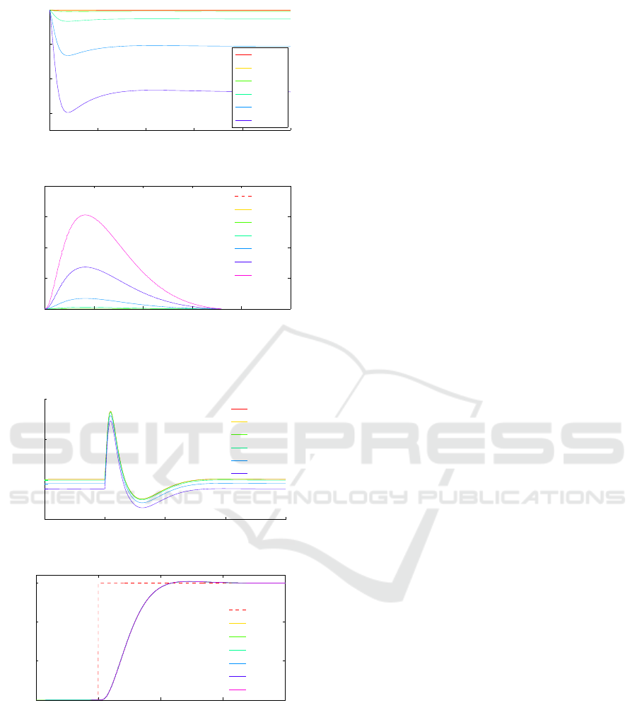
5.1.2 Angular Acceleration Estimation

A frequent problem in estimation is the delay in mea-

surements. Besides the measurements accuracy, it

is important to minimize measurement delay since it

may seriously deteriorate the performance of the con-

trolled system. Additional to these issues, in the case

of our controlled system we observed a different phe-

nomena, as the linear predictor assumes a linear sys-

tem response and gives a very small weight to the ac-

tual measurements. This results in a response esti-

mation which is faster than the real system response,

as presented in ﬁgure 6. This happens because when

adding the η parameter to the INDI implementation,

the resulting linearization is no longer pure, resulting

on a slower response. Closing the loop, we verify that

this slower response leads to a desynchronization be-

tween the estimated angular acceleration and the real

one. As the estimation is faster than the true accelera-

tion, we experimented adding a delay to the estimator.

Figure 7 presents the estimated angular acceleration

for different delay values b, for both open- and closed-

loop scenarios. We can observe that increasing the

estimation delay to b = 2 increases the synchroniza-

tion of the closed-loop response and decreases oscil-

lation. A higher delay results in a response oscillation

increase. The estimation error is still signiﬁcant and

further improvement in the estimation should improve

the closed-loop response.

5.2 Robustness to Model Uncertainties

In order to evaluate the performance of the proposed

sensor-based solution, we will evaluate its robustness

to model uncertainties. In the quadrotor control case,

we will test the only model element that is explicit in

the INDI control law, the matrix of inertia. To repre-

sent the model inaccuracies we will multiply the real

inertia matrix J (used in the quadrotor dynamics sim-

ulator) by a factor σ representing the parameter un-

certainty. The estimated inertia

J = σJ (38)

is the inertia used by the INDI control law.

Assuming perfect sensors, ﬁgure 8 shows the re-

sponse of the controlled system to a step reference in

roll angle. Figure 8(a) presents the system response

when INDI assumes an inertia lower than the real

one. We can observe that for σ = 0.4 (in fact for

0.4 ≤ σ < 1) the controlled system has a response

very close to the nominal one (σ = 1). When σ = 0.3,

the controlled system response shows high frequency

oscillations and for lower values (σ < 0.3) the system

becomes unstable. Figure 8(b) shows that the system

response for σ ≤ 2 is a little more oscillatory, corre-

sponding to a slightly faster response. For σ ≥ 3 we

have a higher overshoot and settling time, which for

higher values of σ may result in the system instabil-

ity. This means that even with an underestimation of

60% or overestimation of 100% of the quadrotor in-

ertia, the INDI controller still shows very little loss of

performance.

Assuming real sensors and including the angu-

lar acceleration estimation, ﬁgure 9 presents the con-

trolled quadrotor response to a 15 deg reference step

in roll angle for different values of σ. We can observe

an evolution similar to the perfect sensors test, with

the controlled response degraded with the higher vari-

ation of the inertia uncertainty. This degradation hap-

pens for smaller inertia errors as we can see in ﬁg. 9(a)

for inertia underestimation and on ﬁg. 9(b) for iner-

tia overestimation. For this more realistic scenario,

we observe that the controlled system performance is

similar for 0.5 ≤ σ ≤ 1.5, corresponding to a smaller

but still signiﬁcant robustness to model uncertainty.

5.3 Sensitivity to Sampling Time

The deduction of the INDI control law lies on the as-

sumption that for a small enough sampling time the

state variation between samples is negligible when

compared to the actuation input. The satisfaction of

this assumption requires in practice that the controller

dynamics be much faster than the quadrotor dynam-

ics. In the following we will check if this holds for our

INDI controller implementation, and how high does

this sampling rate need to be so that INDI is effective.

Figure 10 represents the system response to a

15 deg step in roll, where the chosen base sampling

frequency f

= 100 Hz is limited by the used sensors

set. We can observe that the decrease of the sam-

pling frequency below 50 Hz deteriorates the system

response, presenting a higher overshoot and settling

time. At f

= 20 Hz the system seems close to sta-

bility limits and for lower sampling frequencies the

system becomes unstable. These results show that, as

expected, INDI is sensitive to the controller sampling

frequency.

6 ROBUSTNESS TO WIND

DISTURBANCES

One of the major advantages of INDI is its robustness

to state-only dependent model uncertainties. In air-

craft ﬂight control this is an important characteristic

as the most difﬁcult to identify aerodynamic model

Quadrotor Attitude Control using Incremental Nonlinear Dynamics Inversion

105

2.8 3 3.2 3.4 3.6 3.8

Time (seconds)

roll acceleration (rad/s

)

open loop response

estimated

linear

real

2.8 3 3.2 3.4 3.6 3.8

−5

Time (seconds)

roll acceleration (rad/s

)

closed loop response

estimated

linear

real

Figure 6: Angular acceleration estimation output.

2.8 3 3.2 3.4 3.6 3.8

Time (seconds)

roll acceleration (rad/s

)

open loop response

2.8 3 3.2 3.4 3.6 3.8

−5

Time (seconds)

roll acceleration (rad/s

)

closed loop response

estimated

linear

real

estimated

linear

real

(a) b = 1

2.8 3 3.2 3.4 3.6 3.8

Time (seconds)

roll acceleration (rad/s

)

open loop response

2.8 3 3.2 3.4 3.6 3.8

−5

Time (seconds)

roll acceleration (rad/s

)

closed loop response

estimated

linear

real

estimated

linear

real

(b) b = 2

2.8 3 3.2 3.4 3.6 3.8

Time (seconds)

roll acceleration (rad/s

)

open loop response

2.8 3 3.2 3.4 3.6 3.8

−5

Time (seconds)

roll acceleration (rad/s

)

closed loop response

estimated

linear

real

estimated

linear

real

Figure 7: Estimation output with delay α.

part is grouped with the state-only dependent dynam-

ics, usually requiring extensive work, such as wind

tunnel tests or numeric ﬂuid dynamic simulations.

This is what makes the INDI control algorithm an

attractive choice for ﬂight control architectures, as it

only requires the modelling and identiﬁcation of the

aerodynamics actuation part. This section demon-

strates the INDI robustness to wind disturbances (for

better results visualization, we only present the results

with constant wind).

ICINCO 2017 - 14th International Conference on Informatics in Control, Automation and Robotics

106

2 3 4 5 6

step response − σ < 1

Time (s)

roll (deg)

reference

σ = 1

σ = 0.4

σ = 0.3

(a) σ < 1

2 3 4 5 6

step response − sigma > 1

Time (s)

roll (deg)

reference

σ = 1

σ = 2

σ = 3

σ = 5

(b) σ > 1

Figure 8: Robustness to inertia uncertainty - results assum-

ing perfect sensors.

2 3 4 5 6

step response − σ < 1

Time (s)

roll (deg)

reference

σ = 1

σ = 0.5

σ = 0.4

(a) σ < 1

2 3 4 5 6

step response − sigma > 1

Time (s)

roll (deg)

reference

σ = 1

σ = 1.5

σ = 2

σ = 3

(b) σ > 1

Figure 9: Robustness to inertia uncertainty - results with

angular acceleration estimation.

2 3 4 5 6

step response

Time (s)

roll (deg)

reference

100 Hz

50 Hz

33.3 Hz

20 Hz

Figure 10: Sampling frequency sensitivity test.

As the designed controller only concerns the

quadrotor attitude stabilization, we will only consider

the disturbances in terms of torques, which are de-

scribed by

= D

(39)

where D

is a rotational drag coefﬁcient matrix and

is the true air relative angular rate.

The tests concern the quadrotor response to con-

stant wind steps of different values, namely the con-

troller actuation torque request and respective atti-

tude.

In ﬁgure 11 we present the INDI obtained, namely

the torque request in 11(a) and the quadrotor roll an-

gle in 11(b). The INDI controller shows a quick but

small torque to counteract the wind disturbance. As

a result of this torque, we can observe the roll an-

gle increasing in the ﬁrst 0.2 seconds, followed by

a decrease and stabilization at 0 degrees before the

mark of 0.8 seconds, demonstrating the expected dis-

turbance rejection of this solution.

After the system stabilizes we apply a step of 15

degrees to the roll reference so we can observe if the

quadrotor maneuvers correctly under the wind distur-

bance.

Figure 12 shows the INDI control action request

(ﬁg. 12(a)) to the roll reference step, and respective re-

sponse (ﬁg. 12(b)). The control action shows a small

variation for different wind intensities, guaranteeing

the insensitivity of the roll response to the increase of

the wind intensity.

7 CONCLUSIONS

This paper presents the incremental version of the

nonlinear dynamics inversion control approach, and

applies it to the quadrotor attitude control problem.

The theoretical formulation of INDI is presented

alongside with the NDI formulation for a better com-

parison of approaches. The same is done when the

INDI formulation is applied to the speciﬁc case of

Quadrotor Attitude Control using Incremental Nonlinear Dynamics Inversion

107

0 0.2 0.4 0.6 0.8 1

−0.03

−0.02

−0.01

Time (s)

Torque (Nm)

0 m/s

1 m/s

2 m/s

5 m/s

10 m/s

15 m/s

(a) Torque τ

request

0 0.2 0.4 0.6 0.8 1

0.05

0.1

0.15

0.2

Time (s)

Roll (deg)

ref

0 m/s

1 m/s

2 m/s

5 m/s

10 m/s

15 m/s

(b) Roll response

Figure 11: INDI response to constant wind disturbance.

2.5 3 3.5 4 4.5

−0.1

0.1

0.2

Time (s)

Torque (Nm)

0 m/s

1 m/s

2 m/s

5 m/s

10 m/s

15 m/s

(a) Torque τ

request

2.5 3 3.5 4 4.5

Time (s)

Roll (deg)

ref

0 m/s

1 m/s

2 m/s

5 m/s

10 m/s

15 m/s

(b) Roll response

Figure 12: INDI response to roll step reference with con-

stant wind disturbance.

the quadrotor attitude control. This is done after the

quadrotor model is presented, and it allows us to bet-

ter acknowledge the speciﬁcities of the approaches.

While NDI is a model-based approach, dependent on

an accurate system model, the INDI solution substi-

tutes this model knowledge requirement by accurate

sensor measurements and/or variables estimation, and

high enough sampling times.

For an easier and more straightforward INDI con-

trol design, this paper addresses implementation is-

sues like INDI parameter tuning, linear control de-

sign and angular acceleration estimation. INDI is an

intrinsically integrative control approach, where the

present control action is obtained varying the previ-

ously applied control action. We show that this vari-

ation should be weighted similarly to an integrative

term in PID control, and demonstrate this by simulat-

ing the closed-loop response for different weights.

We demonstrate the INDI robustness to model un-

certainties varying the quadrotor inertia. We show

that, in this case, the INDI approach handles an iner-

tia estimation variation between 0.5 and 1.5 times the

true value, considering real sensors and estimators.

An underlying assumption in INDI is that the con-

troller sampling rate is higher than the system higher

frequency in order to neglect states variation between

samples. A sensitivity analysis to the controller sam-

pling frequency is also done, showing that the INDI

performance is indeed compromised by this parame-

ter choice. However, given the processing capabilities

of today’s processors, the bottleneck for this choice

lies not in the processor capacities but rather on the

acquisition rates of the existing sensors set.

Finally, results demonstrate the robustness of the

solution in the presence of wind disturbances. The

INDI controller not only is able to reject the distur-

bance but is also able to properly follow attitude ref-

erences even with increased wind intensity.

ACKNOWLEDGEMENTS

This work was supported by FCT, through IDMEC,

under projects LAETA (UID/EMS/50022/2013).

REFERENCES

Azinheira, J., Moutinho, A., and Carvalho, J. (2015). Lat-

eral control of airship with uncertain dynamics us-

ing incremental nonlinear dynamics inversion. IFAC-

PapersOnLine, 48(19):69–74.

Bastin, G. (2013). On-line estimation and adaptive control

of bioreactors, volume 1. Elsevier.

Esteves, D., Moutinho, A., and Azinheira, J. (2015). Sta-

bilization and altitude control of an indoor low-cost

quadrotor: design and experimental results. In Proc.

2015 IEEE International Conference on Autonomous

Robot Systems and Competitions, pages 150–155,

Vila Real, Portugal. IEEE.

ICINCO 2017 - 14th International Conference on Informatics in Control, Automation and Robotics

108

Goman, M. and Kolesnikov, E. (1998). Robust nonlinear

dynamic inversion method for an aircraft motion con-

trol. AIAA Paper, pages 98–4208.

Krstic, M., Kokotovic, P. V., and Kanellakopoulos, I.

(1995). Nonlinear and adaptive control design. John

Wiley & Sons, Inc.

Liao, F., Wang, J. L., and Yang, G.-H. (2002). Reliable ro-

bust ﬂight tracking control: an lmi approach. Control

Systems Technology, IEEE Transactions on, 10(1):76–

89.

Mallikarjunan, S. and et al. (2012). L1 adaptive controller

for attitude control of multirotors. In AIAA Guid-

ance, Navigation, and Control Conference, pages 1–

15, Minnesota, USA. AIAA.

Sadeghzadeh, I., Mehta, A., and Zhang, Y. (2011).

Fault/damage tolerant control of a quadrotor heli-

copter UAV using model reference adaptive control

and gain-scheduled PID. In AIAA Guidance, Navi-

gation, and Control Conference, pages 1–13, Oregon,

USA. AIAA.

Sieberling, S., Chu, Q., and Mulder, J. (2010). Robust

ﬂight control using incremental nonlinear dynamic in-

version and angular acceleration prediction. Journal

of guidance, control, and dynamics, 33(6):1732–1742.

Simpl

ıcio, P., Pavel, M., Van Kampen, E., and Chu, Q.

(2013). An acceleration measurements-based ap-

proach for helicopter nonlinear ﬂight control using in-

cremental nonlinear dynamic inversion. Control En-

gineering Practice, 21(8):1065–1077.

Stevens, B. and Lewis, F. (2003). Aircraft control and sim-

ulation. John Wiley & Sons.

Quadrotor Attitude Control using Incremental Nonlinear Dynamics Inversion

109