A Quasi-realistic Internet Graph

Paulo Salvador

DETI, University of Aveiro, Instituto de Telecomunicac¸

oes, Aveiro, Portugal

Keywords:

Internet, Graph Model, Quasi-realistic, Real IX and Submarine Cables.

Abstract:

The existence of a realistic Internet interconnections model has been an important requirement to effectively

support areas as routing optimization, routing security, and services QoS prediction. However, no usable

and no useful models exist. The existing interconnection models are to (i) simplistic to be applicable in real

scenarios, or (ii) incorporate to much uncorrelated information that cannot be used due to its complexity. This

work presents the construction steps and ﬁnal solution for a quasi-realist graph that models the Internet as an

all. The graph is based on all known Internet exchange points (IX) and landing points of all known submarine

cables. The lack of information about interconnections between IX and landing points is extrapolated from

simple rules that take in consideration Earth geographic characteristics. This approach results in a graph that

includes all major corner stones of the Internet while maintaining a simple structure. This graph can then

be used to predict connectivity and routing properties between any two geographical points in Earth. The

proof-of-concept results, even with very simplistic assumptions as similar node and link loads and symmetric

routing by the shortest path, show that the model allows the prediction of the round-trip time of trafﬁc and

number of nodes between any two Internet points with an acceptable average error.

1 INTRODUCTION

Internet complexity in terms of magnitude, unknown

interconnectivity, and asymmetry restricts the con-

struction of any useful and usable model. An Internet

quasi-realist models can be used in routing optimiza-

tion studies, specially when properties of nodes, links

and addressing can be totally controlled while main-

taining a close to real structure of relations. Security

topics, namely the ability to detect and locate sources

of trafﬁc redirection attacks (Pilosov and Kapela,

2008), can greatly beneﬁt from a quasi-realistic In-

ternet relations. Solutions based on constant mo-

torization of round-trip time to a speciﬁc locations

from multiple worldwide location allow the detection

of routing anomalies (Salvador and Nogueira, 2014).

However, such mechanisms rely on an effective Inter-

net model to identify and locate the source of illicit

routing anomalies. Also, when deploying a world-

side scale service based on Content Distribution Net-

works (CDN) it is import to infer a priori the expected

quality of service for users in diverse world locations

and under multiple network conditions.

This paper addresses the construction of an Inter-

net graph model based on real data, such as subma-

rine cables landing points and IX locations, and con-

strained by Earth geographical characteristics. The

resulting graph has an open structure where nodes and

links have properties (e.g., IX name, landing point

name, and geographic distances) and is open to de-

ﬁne other properties (e.g., node load, link load, link

speed, etc. . . ).

The developed code for construction and ﬁnal

and usable Internet graph are publicly available at

graph.netconfs.net.

2 RELATED WORK

Several works on mapping of the Internet have been

presented, however, their are restricted to cataloging

and visualization of Internet nodes and connections.

Durairajan et .al (Durairajan et al., 2013; Durairajan

et al., 2015) constructed a geographic database of the

Internet based on real data, which result is publicly

available (internetatlas.org) and allows data visualiza-

tion and analysis. However, such compilation of data

is easily usable in studies because it requires data ag-

gregations in a valid model that incorporates all inter-

connections and relation

Salvador, P.

A Quasi-realistic Internet Graph.

DOI: 10.5220/0006440100270032

In Proceedings of the 14th International Joint Conference on e-Business and Telecommunications (ICETE 2017) - Volume 1: DCNET, pages 27-32

ISBN: 978-989-758-256-1

3 INTERNET ELEMENTS AND

INTERCONNECTIONS

3.1 Nodes

The Internet graph nodes will be all known IX

and landing points from submarine cables from

data publicly available compiled by TeleGeog-

raphy. Submarine cable information is available

on website TeleGeography Submarine Cable

Map (www.submarinecablemap.com) and re-

spective repository (github.com/telegeography/

www.submarinecablemap.com). Internet exchanged

information is available on website TeleGeography

Internet Exchange Map (internetexchangemap.com)

and respective repository (github.com/telegeography/

www.internetexchangemap.com).

The available data in December 5

2016, listed

1202 IX, however only 600 where considered. IX

from the same provider at the same building or nearby

buildings were merged and considered as a single

IX node. At the same date, there were 368 listed

submarine cables, with a total of 947 unique land-

ing points (considering its identiﬁer and geographi-

cal location). From the 947 unique landing points,

two pairs of nodes had the same identiﬁer but dif-

ferent however close geographic locations. Each of

these pairs of points were merged into a single land-

ing point. Therefore, only 945 landing points nodes

were integrated into the graph.

3.2 Links

Internet link information is almost inexistent. The

only real information must be extracted from the

known submarine cables information, where is pos-

sible to assume that each cable landing point has a di-

rect connection to all other landing points. However,

the publicly available information does not deﬁne the

order by which the landing points are connected, nei-

ther the geographic path that the cable follows. There-

fore, all Internet oceanic links and respective path can

be closely inferred from the available data by impos-

ing constrains has geographic elevation (ocean depth)

and geographic distances between points.

For Internet land links, available information is re-

ally limited by service providers and difﬁcult to corre-

late with IX and landing points locations. Portals like

Internet Atlas have information about some providers

in restricted areas of the world, but is difﬁcult to in-

fer inter-connections between providers. In this work

was choose a more heuristic approach in which land

links were deﬁned based on basic rules constrained

LP2

LP3

LP4 IX3

LP1

IX1

IX2

LP1,LP3,path:[A,B,C,D,E,F,G,H]

LP1,LP4,path:[A,B,C,D,E,F,G,H,I,J,K,L]

LP1,LP2,path:[A,B,C,D,E,F]

LP1,IX1,path:[T,S,M]

IX1,IX3,path:[M,R,Q,P]

IX3,IX2,path:[P,O,N]IX2,LP4,path:[N,X,Y]

IX2,IX1,path:[N,M]

LP2,LP4

path:[F,G,H,I,J,K,L]

LP2,LP3,path:[F,G,H]

LP3,LP4

path:[H,I,J,K,L]

LP3,IX2,path:[V,W,N]

Figure 1: Graph logical representation.

by the maximum number of neighbor nodes within a

geographical range.

4 GRAPH STRUCTURE AND

DYNAMICS

It was assumed that Python is the nowadays language

of election for fast and lightweight development.

Therefore, the Internet graph was constructed using

the Python package NetworkX (networkx.github.io/)

which allows the creation, manipulation, and analysis

of the structure and dynamics of complex networks. It

was chosen a NetworkX Undirected Simple Graph for

modeling the Internet nodes and inter-connections,

because it is assumed that the link properties between

two nodes is the same for both directions.

A NetworkX allows the addition of arbitrary at-

tributes for graph nodes and links. Nodes will an iden-

tiﬁer and two attributes ntype and coord, the ﬁrst

deﬁnes the type of node (IX or Landing Point - LP)

and the second the geographic coordinate as a 2-tuple

with latitude and longitude. Links (or edges under

NetworkX nomenclature) are deﬁned by the two end-

point nodes and have three attributes etype, dist and

path, the ﬁrst deﬁnes the type of the link (Ocean,

Land, Land to Ocean, etc. . . ), the second attribute de-

ﬁnes the geographical distance of the link and the ﬁnal

attribute deﬁnes the geographical path of the link as a

list of geographical coordinates. The unidirectional

nature of the graph implies that the attributes between

node1 and node2, are the same as the ones between

node2 and node1. Therefore, the geographical path

may have to be inverted when starting from the node

considered as the end of the path.

Figure 1 depicts a logical representation of the

graph, where letters represent the geographic coordi-

nates of the respective points.

DCNET 2017 - 8th International Conference on Data Communication Networking

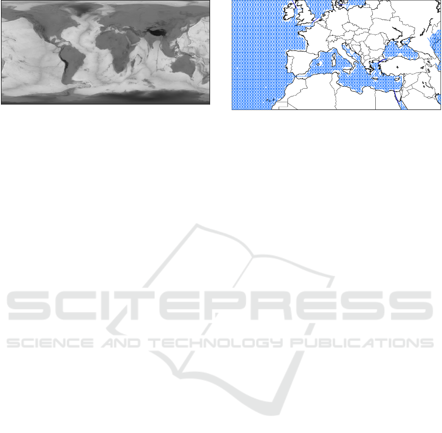
Figure 2: Earth elevation/depth map.

5 GRAPH CONSTRUCTION

Since all considered graph nodes are known they were

just added to the graph with the respective attributes.

The deﬁnition of the links followed the following

steps:

1. For each submarine cable determine the ocean

path between all pairs of landing points. Add a

graph edge for each pair with the respective ocean

path attribute.

(a) For each landing point, determine the closest

ocean grid point (ocean landing point).

(b) Determine its end-points. Which may be more

than two.

endpoints that inter-connects all ocean landing

points.

(d) Add a edge to the Internet graph for each pair of

landing points using as path attribute the ocean

path obtained in step 2.

2. Based on heuristic rules determine the connec-

tions between IX over land paths. Add a graph

edge for each one with the respective land path

attribute.

3. Based on heuristic rules determine the connec-

tions between IX and landing points over land

paths. Add a graph edge for each one with the

respective land path attribute.

4. Solve the cases were a node or a set of connected

nodes (sub-graph) are disconnected from the main

group of nodes.

Steps 1 to 4 require an underlying ocean grid and

land grid to determine the paths. This grids were de-

ﬁned also as unidirectional NetworkX graphs to allow

the estimation of the best paths in ocean or land.

Both ocean and land grids were constructed based

on elevation/depth information obtained from a geo-

graphic referenced tiff from the USA National Ocean

and Atmospheric Administration (NOAA) depicted

Figure 3: Ocean grid.

in Figure 2. All geographic distances were calcu-

lated over the Earth Rhumb line between two loca-

tions (see. Appendix).

The ocean grid construction started by deﬁned a

set of geographic underwater points from latitude -

to 78

, and from longitude -180

to 180

in one

degree intervals. An Ocean Grid edge is included

if both end-points are underwater and three equally

spaced points between them are also underwater. A

georeferenced point is considered underwater if its

(average) elevation is zero or less. This rule may er-

roneously include land locations that are below sea

level (e.g., Netherlands), and erroneously exclude lo-

cations, subject to high tides, that are not permanently

covered by water. Moreover, the choice to consider

zero elevation has threshold for allow the passage of

a submarine cable was a conscious one; to compen-

sate the low resolution (high distance between grid

georeferenced points) that was excluding most of the

water straits and channels of the world were subma-

rine cables pass. Even with this relax elevation rule

some important water straits and channels were not

considered viable to pass a submarine cable and had

to be manually added. Namely:

• Add connection over the Suez channel.

• Add connection over the Panama Chanel.

• Add connection over the English Chanel.

• Add connection near Isle of Man Channel (Irish

Sea to Atlantic North).

• Add connection between the sea channel between

Denmark and Sweden.

• Add connection from the White Sea to Barents

Sea in Russia.

• Add connection from Mediterranean Sea to Istan-

bul and Black Sea, over Dardanelles strait and Sea

of Marmara.

• Add connection over Malacca strait between

Malaysia and Indonesia Sumatra Island.

• Add connection over the strait between Indone-

sian islands of Sumatra and Java.

A Quasi-realistic Internet Graph

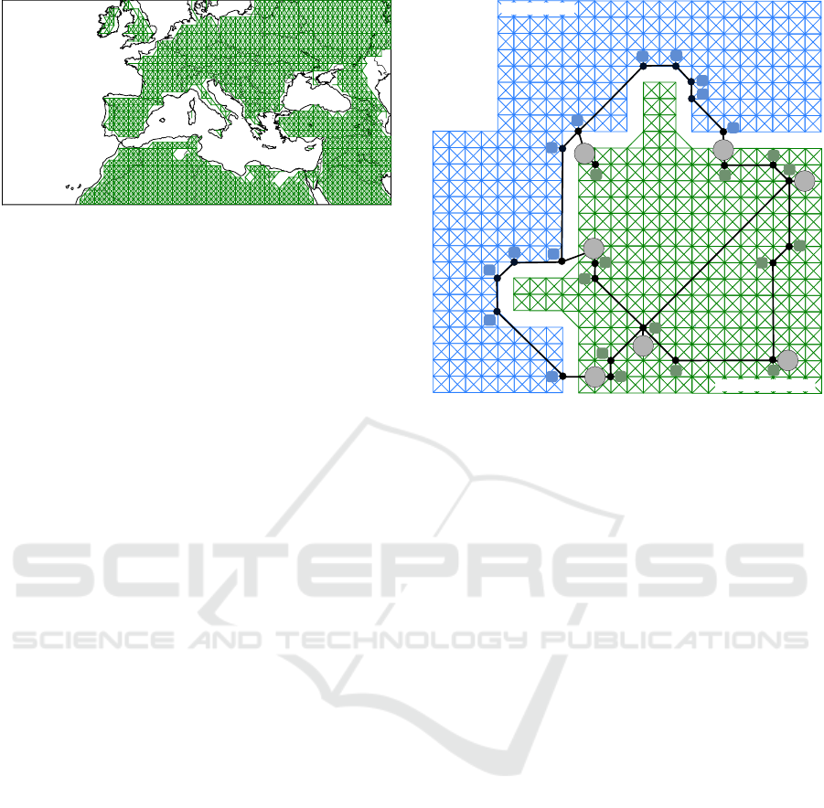
Figure 4: Land grid.

Moreover some points of Ocean Grid located in

Netherlands had to be removed because they were

classiﬁed as underwater, because they are below the

sea level however are dry land. The resulting ocean

grid had only one unconnected subgraph (isolated

ocean zone), namely the Caspian Sea with 80 nodes.

The ﬁnal ocean grid had 31434 nodes and 119229

edges. Figure 3 depicts a zoom area of the ocean grid

that includes the Atlantic ocean, seas of the north of

Europe, Mediterranean sea at the south and part of the

Caspian sea. Note that, in the ﬁgure is visible some of

the manual edge additions, namely the Panama Chan-

nel, around great Britain islands, between Denmark

and Sweden and from Mediterranean Sea to Istanbul.

he construction of the Land Grid followed a sim-

ilar approach using as rule for a grid points and in-

termediary point an elevation higher then zero. It in-

cluded geographic points above sea level points from

latitude -80

to 80

, and from longitude -180

to 180

in one degree intervals. Only two major faults on the

grid had to be corrected, namely the addition of long

bridges (e.g., between three of Japan main islands)

that transport terrestrial data cables. Namely:

• One connection between Honshu and Kyushu is-

lands in Japan.

• One connection between Honshu and Hokkaido

islands in Japan

The ﬁnal land grid had 18312 nodes and 65690 edges.

Figure 4 depicts a zoom area of the land grid that in-

cludes Europe and the north of Africa.

Figure 5 depicts an simple network example that

will illustrate the Internet graph construction process

that should lead to a resulting graph similar to the one

depicted in Figure 1. The Step 1 of the Internet graph

construction consists in, for all submarine cables, add

a graph edge for all landing point pairs in a cable us-

ing an ocean path. In step 1a, is determined the closest

point of the ocean grid to each landing point. Using

Figure 5 as an example, landing points LP1, LP2, LP3

and LP4 are associated with points A, F, H, and L of

the Ocean grid, respectively. In step 1b, are deter-

mined the two points with the higher distance between

LP2

LP1

LP4

Ocean Grid

Terrestrial Grid

IX2

IX1

IX3

LP3

Figure 5: Ocean and terrestrial grids usage example.

them, these will be considered the main end-points

of the cable (LP1 and LP4 in the example). Note

that, there are submarine cables with more than two

end-points. In step 1c, is determined the order and

path by which the landing points are inter-connected.

Starting from one of the main end-points of the ca-

ble, the algorithm searches the closest landing point,

and the respective ocean points, using the ocean grid

and determines the geographic path. From this new

point searches for the remaining landing points the

closest one, and so one until the other main end-point

is reached. In the example, starting from LP1 ocean

grid point A, the closest ocean point by ocean is F,

therefore the next landing point of the cable with be

LP2 using the Ocean path [A,B,C,D,E,F]. Then from

LP2 ocean grid point F, the closest ocean point by

ocean is H, therefore the next landing point of the ca-

ble with be LP3 using the Ocean path [F,G,H], and

so on until LP4 is reached. However in this process,

due to the existence of multiple end-points or intri-

cate cable paths, some landing-points may be left un-

connected. To discover how they inter-connect to the

remaining cable landing points, a similar algorithm

is used; for all pairs of connected and unconnected

landing points calculate the pair with the shortest dis-

tance over ocean and connect them; repeat until all

nodes are connected. In Step 1d, for all pairs of a

landing points in a cable is added edge to the Inter-

net graph using as path attribute the concatenation

of geographic paths obtained from the order of inter-

connection and paths obtained in step 1c.

The heuristic rules for construction steps 2 and 3

used were: (i) each IX connects to a maximum of

12 IX neighbors within a 2500Km radius using land

DCNET 2017 - 8th International Conference on Data Communication Networking

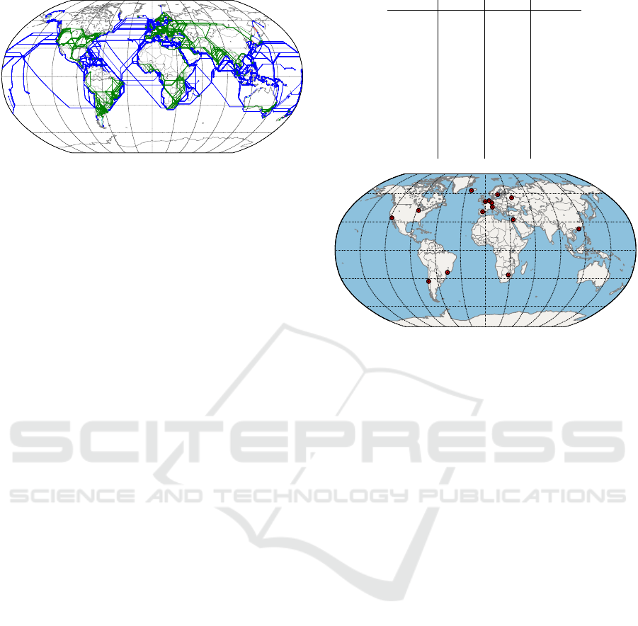
Figure 6: Final quasi-realistic Internet graph.

paths, (ii) each landing point connects to a maximum

of 3 IX within a radius of 250km using a land path,

and (iii) unconnected subgraphs are joined to the mas-

ter graph by selecting the node closest to a main graph

node within 2000Km using a land path. Large dis-

tances are required to allow the inter-connection of

IX in South America and Africa where they are more

further apart. The determination of the land paths be-

tween nodes starts by inferring the closest land grid

point to each location, and ﬁnd the shortest path us-

ing the land grid graph. In the example, IX2 connects

to LP3 and LP4, from its land grid point N using paths

[N,W,V] to LP3 and [N,X,Y] to LP4.

Finally in step 4, the unconnected nodes or sub-

graphs were merged with the main graph with a di-

rect connection (not using the ocean or land grids)

between the node closest to a main graph node and

the respective closer node within 500Km. It was nec-

essary to extend the maximum range of direct connec-

tions to 2000Km, to include a connection in Sacalina

Island, Russia to inter-connect the ”Far East Subma-

rine Cable System” to the remaining nodes.

The ﬁnal Internet graph constructed as 1545 nodes

(600 IX, and 945 Landing Points), and 10332 edges.

Figure 6 depicts the Internet graph in a world map.

6 PROOF-OF-CONCEPT

RESULTS

To validate the constructed Internet graph a simple ex-

periment was devises to see how the model allow the

prediction of round trip time (RTT) and number of

hops, between multiple location on Earth assuming

simplistic simpliﬁcations as link and node loads uni-

formity and routing symmetry using the shortest path.

For the measurements it were used 15 servers spread

all over the world, see Figure 7. Measurements were

made over a period of one week (from March 10

March 17

2017) using ping and traceroute, re-

spectively.

Table 1 presents the measured (at the left) values

City Country Latitude Longitude

Amsterdam Netherlands 52.3702157 4.8951679

Chicago US 41.8781136 -87.6297982

Frankfurt Germany 50.1109221 8.6821267

Hafnarfjordur Iceland 64.0291054 -21.9684626

Hong-Kong China 22.396428 114.109497

Johannesburg South Africa -26.2041028 28.0473051

LA US 34.0522342 -118.2436849

London UK 51.5073509 -0.1277583

Madrid Spain 40.4167754 -3.7037902

Milan Italy 45.4654219 9.1859243

Moskow Russia 55.755826 37.6173

ao Paulo Brazil -23.5505199 -46.6333094

Stockholm Sweden 59.3293235 18.0685808

Tel Aviv Israel 32.0852999 34.7817676

na del Mar Chile -33.0153481 -71.5500276

Figure 7: Test server locations.

for the average RTT in milliseconds (top) and number

of nodes (bottom).

Using the Internet graph model it was estimated

the path distance between all servers and the number

of nodes. Assuming a speed of data propagation of

60% of the speed of light it was possible to estimate

the RTT between two points. Table 1 presents the pre-

dicted (at the right) values. The average absolute error

of prediction was approximately 28.8% for the RTT

and 36.1% for the number of nodes. To comparison,

the average absolute predicting the RTT using the di-

rect line geographic distance between any two points

(and the same speed of data propagation) were 48.3%.

7 CONCLUSIONS

This paper presented the construction process and ﬁ-

nal result of a quasi-realistic Internet graph that incor-

porates real infrastructure data. Such graph will allow

the optimization and prediction of services that oper-

ate in a world-scale environment. A simple experi-

ment with the graph proved that large gains in terms

of prediction of Internet end-to-end metrics can be

achieve. Moreover, the graph (and associated usage

and construction code) is publicly available and can

be expanded with additional Internet information.

As future work, the graph may be improved with

localized Internet topology information made avail-

able by ISP, and with additional measurements (new

or historic ones available in public repositories).

A Quasi-realistic Internet Graph

Table 1: Measured (left) and predicted (right) values for the average RTT in milliseconds (top) and number of nodes (bottom)

between multiple locations.

Amsterdam

Chicago

Chile

Frankurt

Hong-Kong

Iceland

Israel

Johannesburg

London

Madrid

Milan

Moskow

ao Paulo

Sweden

Amsterdam - 103.0/130.0

13/13

204.9/208.8

18/15

18.0/9.9

5/5

309.1/177.7

12/19

36.1/39.6

6/6

65.2/87.8

8/15

172.7/208.6

8/18

153.4/174.7

12/18

6.5/7.4

13/5

31.5/29.7

7/7

24.1/21.6

7/8

46.3/49.6

5/12

231.8/171.4

12/12

22.8/36.9

6/10

Chicago 103.1/130.0

12/13

- 139.7/157.6

19/12

109.1/133.2

14/14

206.1/300.9

19/28

124.9/166.0

13/16

159.2/211.0

16/24

261.2/289.7

16/17

66.8/46.0

15/6

96.3/123.1

17/9

110.7/133.5

14/10

112.3/136.9

16/13

149.9/172.9

17/21

144.9/167.9

13/13

118.1/152.6

13/14

Chile 467.7/208.8

16/15

142.5/157.6

19/12

- 216.2/207.9

22/14

472.3/371.1

17/27

588.7/244.2

13/17

216.3/281.2

17/23

763.5/206.1

19/11

178.0/157.4

18/11

700.2/206.4

16/15

225.1/182.6

21/10

220.8/203.2

13/12

392.2/245.0

14/21

255.2/43.5

16/5

272.3/236.0

15/20

Frankurt 6.9/9.9

7/5

109.8/133.2

14/14

214.5/207.9

20/14

- 311.2/168.3

22/15

48.3/43.1

9/6

66.1/78.4

10/11

200.6/199.2

12/14

157.0/177.9

17/19

15.5/10.7

15/6

29.7/29.0

9/6

16.3/12.3

11/4

42.4/40.2

4/8

237.5/170.5

15/11

20.7/44.0

5/11

Hong-Kong 307.0/177.7

12/19

189.0/300.9

14/28

327.5/371.1

23/27

304.1/168.3

24/15

- 314.6/210.8

13/20

349.7/131.4

17/8

434.3/230.3

15/11

160.9/217.3

13/4

271.6/178.4

15/20

267.7/192.1

24/19

283.1/172.7

13/16

316.0/141.3

14/9

324.5/333.7

16/24

309.9/159.9

15/14

Iceland 35.9/39.6

6/6

124.7/166.0

14/16

244.8/244.2

19/17

47.7/43.1

11/6

299.0/210.8

15/20

- 112.7/120.9

13/16

238.5/241.7

12/19

178.7/210.8

17/21

40.1/43.5

13/8

64.2/65.2

11/9

50.5/54.8

9/9

86.4/82.8

9/13

230.0/206.8

13/14

64.0/73.0

13/13

Israel 65.3/87.8

7/15

159.6/211.0

18/24

407.1/281.2

19/23

64.7/78.4

8/11

343.4/131.4

17/8

109.0/120.9

10/16

- 241.1/113.7

11/8

211.0/255.8

11/29

64.6/88.5

13/16

105.1/102.2

10/15

76.1/82.8

12/12

115.2/52.1

7/6

267.4/243.8

14/20

87.1/70.2

9/10

Johannesburg 183.2/208.6

7/18

260.1/289.7

15/17

388.9/206.1

20/11

246.0/199.2

12/14

444.9/230.3

14/11

239.1/241.7

10/19

244.2/113.7

11/8

- 337.6/320.1

18/18

176.1/209.3

11/19

202.8/159.8

9/9

204.6/203.6

10/15

237.9/172.9

8/9

367.1/168.7

12/8

205.3/190.7

14/13

LA 156.9/174.7

11/18

70.7/46.0

14/6

174.7/157.4

21/11

152.4/177.9

20/19

151.4/217.3

12/4

177.2/210.8

12/21

217.5/255.8

15/29

351.9/320.1

18/18

- 195.4/167.9

18/14

178.6/178.2

23/15

176.4/181.7

10/18

193.7/217.6

11/26

177.3/167.7

15/12

185.9/197.4

13/19

London 6.4/7.4

11/5

87.8/123.1

17/9

235.8/206.4

26/15

15.2/10.7

10/6

259.2/178.4

15/20

40.1/43.5

13/8

70.1/88.5

14/16

176.4/209.3

12/19

158.2/167.9

19/14

- 35.1/27.4

14/7

21.8/22.4

13/9

44.6/50.4

12/13

184.4/169.1

17/12

28.6/30.1

12/6

Madrid 31.5/29.7

9/7

110.8/133.5

15/10

224.8/182.6

20/10

27.2/29.0

10/6

271.3/192.1

10/19

64.2/65.2

11/9

107.7/102.2

11/15

203.0/159.8

13/9

172.6/178.2

18/15

35.2/27.4

10/7

- 24.4/23.5

11/4

72.9/66.1

13/13

223.6/145.2

16/7

53.5/56.9

8/12

Milan 19.7/21.6

13/8

112.2/136.9

18/13

223.0/203.2

23/12

16.5/12.3

13/4

288.1/172.7

16/16

50.5/54.8

9/9

68.6/82.8

13/12

204.3/203.6

11/15

168.0/181.7

17/18

22.9/22.4

12/9

24.4/23.5

8/4

- 51.4/46.6

10/10

223.9/165.8

13/9

36.5/50.5

12/13

Moskow 52.2/49.6

5/12

149.2/172.9

18/21

270.0/245.0

23/21

42.0/40.2

7/8

325.2/141.3

17/9

83.6/82.8

10/13

122.4/52.1

8/6

235.1/172.9

10/9

197.3/217.6

18/26

44.5/50.4

13/13

72.7/66.1

9/13

57.8/46.6

10/10

- 267.4/207.6

14/18

65.6/25.8

6/6

ao Paulo 233.5/171.4

11/12

144.6/167.9

18/13

406.5/43.5

16/5

241.3/170.5

21/11

330.4/333.7

20/24

236.5/206.8

12/14

273.4/243.8

16/20

370.8/168.7

14/8

174.5/167.7

19/12

184.1/169.1

18/12

224.0/145.2

21/7

221.6/165.8

12/9

262.9/207.6

13/18

- 228.4/198.6

18/17

Sweden 22.8/36.9

6/10

113.9/152.6

13/14

232.2/236.0

24/20

20.6/44.0

6/11

314.8/159.9

17/14

64.2/73.0

11/13

89.0/70.2

9/10

205.1/190.7

13/13

177.5/197.4

16/19

28.1/30.1

12/6

53.4/56.9

7/12

39.5/50.5

11/13

75.7/25.8

6/6

225.5/198.6

14/17

ACKNOWLEDGEMENTS

This work was supported by the Fundac¸

ao para

encia e Tecnologia (FCT) through PTDC/EEI-

TEL/5708/2014 and UID/EEA/50008/2013.

REFERENCES

Durairajan, R., Barford, P., Sommers, J., and Willinger, W.

(2015). Intertubes: A study of the us long-haul ﬁber-

optic infrastructure. SIGCOMM Comput. Commun.

Rev., 45(4):565–578.

Durairajan, R., Ghosh, S., Tang, X., Barford, P., and Eriks-

son, B. (2013). Internet atlas: A geographic database

of the internet. In Proceedings of the 5th ACM Work-

shop on HotPlanet, HotPlanet ’13, pages 15–20, New

York, NY, USA. ACM.

Pilosov, A. and Kapela, T. (2008). Stealing The Internet

- An Internet-Scale Man In The Middle Attack. In

DEFCON16.

Salvador, P. and Nogueira, A. (2014). Customer-side detec-

tion of internet-scale trafﬁc redirection. In 16th Inter-

national Telecommunications Network Strategy and

Planning Symposium (NETWORKS 2014).

APPENDIX

Geographic Distance over Earth Rhumb Line

Considering two geographic points with latitude ψ

and longitude λ

(in degrees), and latitude ψ

and lon-

gitude λ

(in degrees). The geographic coordinates

for both points in radians are given by:

(ψ

,λ

) = (ψ

π/180,λ

π/180)

(ψ

,λ

) = (ψ

π/180,λ

π/180)

The longitude difference using the shortest route

(East to West, or West to East) is given by:

∆λ = min (mod(λ

− λ

,2π),mod(λ

− λ

,2π))

And the latitude difference is given by:

∆ψ = ψ

− ψ

The projected latitude difference is given by:

∆φ = ln



tan(ψ

/2 + π/4)

tan(ψ

/2 + π/4)



The geographic distance over a Rhumb line is then

given by:

d =







cos(ψ

)

∆λ

+ ∆ψ

, if ∆φ < ρ



∆ψ

∆φ



∆λ

+ ∆ψ

, otherwise

where R is the mean radius of Earth (6371 Km) and ρ

must be the smallest number resolution (e.g., 10

−20

A close to zero projected latitude difference (∆φ < ρ)

means that the path between the points is parallel to

the equator line.

DCNET 2017 - 8th International Conference on Data Communication Networking