Considerations on 2D-Bin Packing Problem: Is the Order of

Placement a Relevant Factor?

Gia Thuan Lam

, Viet Anh Ho

and Doina Logofătu

Vietnamese-German University, Le Lai Street, Hoa Phu Ward, Thu Dau Mot City, Binh Duong Province, Vietnam

Frankfurt University of Applied Sciences, Nibelungenplatz 1, Frankfurt am Main, Germany

Keywords: 2D Bin Packing, Order of Placement, Placement Algorithm, Optimization Techniques, First-Fit, Area

Decreasing Order.

Abstract: The problem of packing a given sequence of items of 2-dimensional (2D) geometric shapes into a minimum

number of rectangle bins of given dimensions is called the 2D bin packing problem. This problem has

various applications across many industries such as steel-, paper- and wood- industries where objects of

certain shapes are needed to be cut from large rectangle panels with the most efficient use of materials. This

problem, however, belongs to the class of NP-Hard problems, implying that no perfect solution exists. Many

proposed solutions involve the use of advanced metaheuristic search techniques such as Local Search,

Simulated Annealing or Genetic Algorithm, but most of them are still greedy-based, which means some

greedy technique such as First-Fit is still used as their core placement algorithm and optimization techniques

are employed only to search for a good ordering or orientation (rotation angles) of the objects so that the

placement procedure can yield the best possible results. Practice has shown that greedy placement algorithm

on the simple area decreasing order can produce excellent results comparable to those on orderings

generated from advanced optimization techniques. This paper discusses the relevance of the order of

placement in the 2D bin packing problem.

1 INTRODUCTION

The 2-dimensional (2D) bin packing is the problem

of packing a list of objects of different geometric

shapes into rectangle bins of fixed dimensions while

minimizing the number of used bins (Lodi et al.,

2010). It is related to many important problems

across a variety of practical areas. In steel industry,

for example, to cut out metal components of

different shapes from a metal sheet, the engineers

always try to minimize the wasted material that will

be thrown away. This problem is a generalization

from the well-known 1D packing problem and can

be generalized to even higher dimensions such as 3D

packing problem which has important applications

in transportation or delivery service where all items

should be transferred using as few vehicles as

possible. Let’s consider the following example.

A hand-made shop needs to produce some

objects of metal in different shapes. These objects

will be used to decorate their new store. This shop

always buys metal panels in forms of rectangle of

fixed dimensions and the objects must be cut from

them in a way that the amount of wasted material

can be minimized.

Figure 1 shows an example where the shop wants

to produce 20 objects of different shapes. A simple

but inefficient placement of objects as shown in

figure 1 costs 3 panels of metal and the wasted area

(blank area) is large. As a result, it makes the price

of material much more expensive.

Figure 1: Example for simple placement.

Figure 2 shows a better placement in which the

280

Lam, G., Ho, V. and Logofatu, D.

Considerations on 2D-Bin Packing Problem: Is the Order of Placement a Relevant Factor?.

DOI: 10.5220/0006440302800287

In Proceedings of the 7th International Conference on Simulation and Modeling Methodologies, Technologies and Applications (SIMULTECH 2017), pages 280-287

ISBN: 978-989-758-265-3

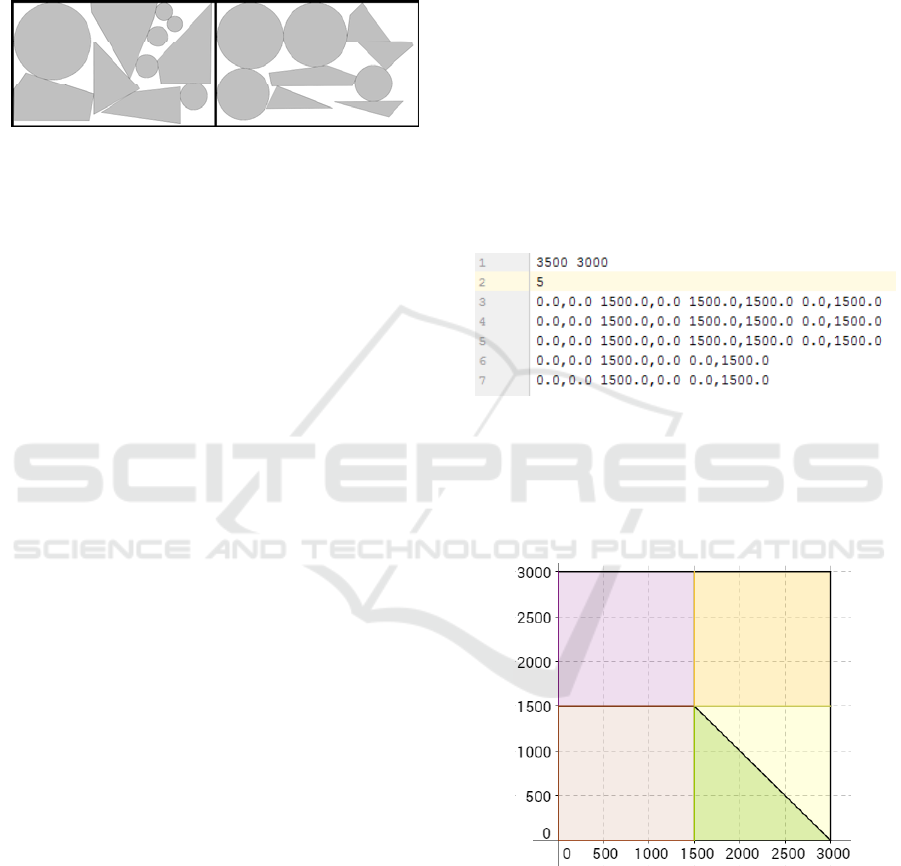
number of panels can be reduced to 2, which is

visually an optimal solution. The wasted area is

much smaller compared to that in figure 1. That

means the material has been utilized efficiently. In

mass production, the amount of saved material may

be significant and generate a huge economic value.

Figure 2: A better placement for items from figure 1.

Due to its large application domain, 2D bin

packing has been one of the core research topics for

many years. However, in computational complexity

theory, it is a combinatorial NP-hard problem.

Hence no optimal deterministic algorithms exist.

Although many sophisticated algorithms have been

developed for it, naïve and simple greedy

approaches such as Best-Fit and First-Fit (Dósa and

Sgall, 1998) strategies seem to yield very good

results in practice compared to those using advanced

search techniques such as Local Search, Simulated

Annealing or Evolutionary Approaches, leading us

to the question whether those advanced techniques

are useful in this problem.

Analyzing many previous algorithms, we

recognize that numerous algorithms in this topic

followed a common pattern. They only concentrated

on improving the order of placement of objects. That

is the sequence deciding which objects should be

placed before others. This paper will demonstrate

that the order of placement it not a useful factor in

solving this problem by testing the First-Fit

algorithm on some random permutations of objects

and comparing the results with that of the area

decreasing order. The reason why First-Fit, a naïve

and simple algorithm, is used and why the area

decreasing order is used as a standard for

comparison will be shown in section 3. In section 4,

an implementation of the First-Fit algorithm will be

presented and most importantly, experimental results

to prove our claim will be presented in section 5.

2 PROBLEM DESCRIPTION

The 2D bin packing is divided into 2 main branches:

one only concerned with rectangle objects, namely

regular bin packing, and the other concerned with

both rectangle and non-rectangle objects called

irregular bin packing which is the focus of our study.

A solution to this problem will process a set of n

objects, each is represented as a sequence of points

= {p

, p

… p

} for some k forming a polygon

of k vertexes and 1 ≤ i ≤ n, and output a placement

of objects inside rectangle bins of given dimensions.

The placement must satisfy the condition that no two

objects intersect with each other and the number of

bin used must be as minimal as possible.

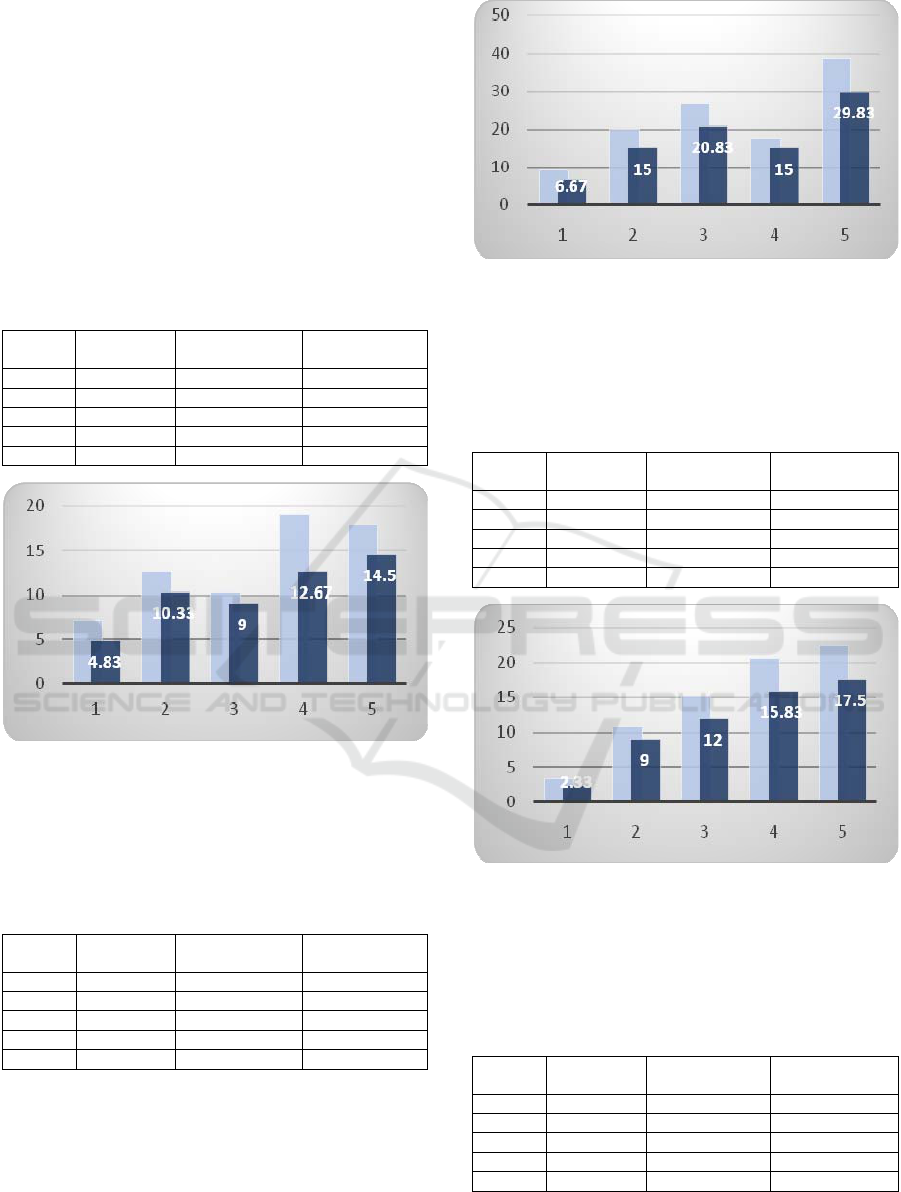
Figure 3 and figure 4 shows an example of the

input and output of a 2D bin packing algorithm,

respectively. The first line of the input gives

dimensions, the width and height of all rectangle

bins, the second line represents the number of items

to place n, followed by n lines, each of which

describes an item as a polygon by listing a sequence

of points.

Figure 3: Sample input for 5 items.

The output in figure 4 is simply a graphical

visualization of an optimal placement. In this case,

we only need 1 bin, which is also an optimal

solution.

Figure 4: Sample output for the placement of 5 items.

Unlike the above example where an optimal

solution can be found easily, the complexity of this

problem in theory is NP-Hard, implying that it is

only possible to find a good approximation in

general case.

Considerations on 2D-Bin Packing Problem: Is the Order of Placement a Relevant Factor?

281

3 BACKGROUND

Both the regular and irregular 2D bin packing

problems have been intensively studied (Lodi et al.,

2002; Bennell et al., 2008). Albeit it is impossible to

solve this problem optimally, numerous efficient

solutions have been proposed and proved extremely

sufficient in practice, especially for the regular

version. The most fundamental but also an excellent

approach in practice is the First-Fit algorithm.

Although a variety of more advanced algorithms

using complicated optimization techniques such as

Local Search (Alvim et al., 1999), Simulated

Annealing (Rao and Iyengar, 1994) or Evolutionary

Algorithm (Junkermeier, 2015) have been

developed, the majority are still based on some

greedy algorithm like First-Fit as the placement

procedure. Different search techniques are

commonly used only to find a good ordering or

orientation (rotation angles) of objects so that the

core placement procedure can produce the best

possible result.

Ferreira (2015) tested the First-Fit algorithm with

1 heuristic and 3 different metaheuristics: First Fit

on area decreasing order (FFD), local search (LS),

simulated annealing (SA) and genetic algorithm

(GA). His experimental results imply a hidden but

disappointing fact that there is almost no distinction

in efficiency among the 4 algorithms regardless of

their varying levels of complexity. Table 1

summarizes his experimental results. N is the

number of objects for input. From his original data,

for each value of N, there are 6 classes of test cases.

Nonetheless, due to the limitation of space, table 1

only stores the average value of all tests of 6 classes

for each input of size N of each algorithm.

Table 1: Summary of Ferreira’s experimental results.

N FFD LS SA GA

20 3.78 3.69 3.62 3.65

40 6.96 6.93 6.84 6.94

60 10.34 10.18 10.20 10.38

80 13.87 13.68 13.72 14.13

100 16.35 16.11 16.20 16.70

From the table, the maximum difference between

any two algorithms given the same input size is less

than 0.59. The bigger the input size, the worse SA

and GA get compared to others, whilst for LS and

FFD, they get better with larger input size.

Nonetheless, considering the complexity of LS, SA

and GA, their performance was so poor compared to

that of FFD, which is not explained in the paper and

becomes the inspiration for our paper to discover

why they are so inefficient. After careful analysis, a

common pattern among these 4 algorithms is that

their optimization objective was only the order of

placement, leading to the question if that is the

problem making advanced optimization techniques

so inefficient. To investigate that question, we repeat

his experiment but only use the FFD as the standard

and compare it against First-Fit on random orderings

of input instead of those generated from advanced

search methods. The reason why First-Fit is chosen

is because of its simplicity and usefulness in

practice, and why area decreasing order is

considered as the standard is already explained by

data from table 1. If random orderings are also good

comparatively to the area decreasing ordering, it is

obvious that there should be no further investigation

into the order of placement in further researches on

this topic.

4 IMPLEMENTATION OF THE

PLACEMENT ALGORITHM

After careful consideration, the core placement

strategy of our study has been decided to be First-Fit

algorithm. For the sake of convenience, we employ

the open source Java implementation of Baly (2016)

which is a variant of First-Fit algorithm. His

implementation is, however, not very optimized and

likely to produce non-optimal results that are too far

from optimality, which may badly affect the

experiment. Therefore, the implementation needs

improving to meet our needs. Firstly, an overview of

his original algorithm will be presented in subsection

4.1. Some improvements will be made and shown in

subsection 4.2 and 4.3. Finally, in subsection 4.4, a

comparison between our improved version and the

original version will be presented to verify if it can

produce acceptable results for the main experiment.

4.1 Overview of the Original Algorithm

The idea of the algorithm is to apply regular bin

packing algorithm for irregular bin packing by

considering that each non-rectangle object is

bounded by a rectangle box which will be treated as

the object itself. By so doing, we can utilize the

advances in regular packing, the field in which

researches have already reached a high level of

maturity (Jylänki, 2010), for the newer field of

irregular bin packing. In regular packing, there are

better alternative techniques, but for the sake of

simplicity, the strategy used in this study is still

First-Fit.

SIMULTECH 2017 - 7th International Conference on Simulation and Modeling Methodologies, Technologies and Applications

282

The first feature is named “try and replace”.

Each bounding box is a rectangle but it is not solid.

The object inside it may leave some free space large

enough to store some smaller objects. By

rearranging objects that have already been placed

(putting smaller ones into bigger bounding boxes),

more empty space can be created. This feature gives

more opportunities of being placed in the current bin

to those objects that fail to be placed by First-Fit.

Last, but not least, the most important feature is

the “gravity system” which simulates real gravity

and directs all objects towards the top-left corner.

The use of this feature is of paramount importance in

that it can compress all currently placed objects

inside a bin to create more free space so that more

objects can be considered. Another use of this

feature is to randomly “drop” objects into the bin

like throwing balls into a container and they will

automatically roll around to find their place. Figure

5 shows the pseudocode for the whole algorithm.

While SomeObjectsAreLeft do

Create new bin

While TheCurrentBinNotFull do

For each object p left do

If FirstFit(p) = success then

continue

endIf

endFor

call TryAndReplace()

call GravitySystem()

drop objects randomly

endWhile

Figure 5: Pseudocode for The Algorithm.

Many optimizations can be done for this

algorithm, two of which will be shown in the next

two subsections 4.2 and 4.3.

4.2 Minimum Bounding Box

The first place that needs improving is the idea of

treating the bounding box of each object as the

object itself. There is no problem with that idea, but

the technique for finding the bounding box

employed in the original algorithm by only finding

the highest and lowest vertical coordinates and the

leftmost and rightmost horizontal coordinates in the

set of vertexes is too trivial and unlikely to generate

acceptable results. Instead of finding any bounding

box, the minimum bounding box in which the

wasted area is minimal should be preferred. It can be

found by rotating the objects through all angles of

integer value from 1 to 180 degree, and selecting the

best one after each rotation using the old method.

This is known as the minimal enclosing box problem

(O'Rourke, 1985).

4.3 Nested Testing to Emphasize

Current Order of Placement

The original implementation is inefficient in the way

that the order of placement is underestimated. An

object failing the First-Fit strategy the first time does

not mean it has no chance of being placed and

should be put behind those coming after it in the

initial order. The positions of “try and replace” and

“gravity system” cannot utilize their full potential of

creating opportunities for each object. Each object

should be given more opportunity of being placed by

those features right after failing the First-Fit

strategy. By so doing, the likelihood of the current

object being added will increase, which may reduce

additional use of new bins. As a result, the order of

placement can be enhanced. Figure 6 shows the

pseudocode for the new version from figure 5. The

difference lies in the positions of “try and replace”

and “gravity system”. They are nested inside the

same loop with the First-Fit strategy and right after

the First Fit strategy fails.

While SomeObjectsAreLeft do

Create new bin

While TheCurrentBinNotFull do

For each object p left do

If FirstFit(p) = success then

continue

endIf

call TryAndReplace()

call GravitySystem()

If FirstFit(p) = success then

continue

endIf

endFor

call GravitySystem()

drop objects randomly

endWhile

Figure 6: Pseudocode for the New Algorithm.

These modifications should be enough to

produce acceptable results for our main experiment.

A comparison by experimental results between the

original and the improved version is shown in

subsection 4.4.

4.4 Comparison between the Old and

New Implementation

In this study, 120 test cases representing 4 classes of

Considerations on 2D-Bin Packing Problem: Is the Order of Placement a Relevant Factor?

283

objects, Stars, Polygons, Circles and Mixed (all of 3

types), are randomly and independently constructed

for experiment. Each class is consisted of 30 tests

and is further divided into 5 subclasses in relation

with their input sizes of 20, 40, 60, 80 or 100 items.

This set of test cases will also be used for section 5.

Table 2, 3, 4, 5 will show the average number of bin

used for input of type Star, Polygon, Circle and Mix,

respectively. Following right after each table is its

corresponding bar chart illustrating its data. In this

case, only the area decreasing order is considered.

Table 2: Average number of used bins for input of type

Star.

Index

Number of

items

Original

Version

Improved

Version

1 20 7.17 4.83

2 40 12.67 10.33

3 60 10.33 9.00

4 80 19.00 12.67

5 100 17.83 14.50

Figure 7: Visualisation of the results for input of type Star

(average of used bins) from Table 2. The original

algorithm – light grey and our modified algorithm – dark

grey. X-axis: simulation number (20 to 100 items, step

20), Y-axis: average number of used bins.

Table 3: Average number of used bins for input of type

Polygon.

Index

Number of

items

Original

Version

Improved

Version

1 20 9.33 6.67

2 40 19.99 15.00

3 60 26.67 20.83

4 80 17.67 15.00

5 100 38.83 29.83

Figure 8: Visualisation of the results for input of type

Polygon (average of used bins) from Table 3. The original

algorithm – light grey and our modified algorithm – dark

grey. X-axis: simulation number (20 to 100 items, step

20), Y-axis: average number of used bins.

Table 4: Average number of used bins for input of type

Circle.

Index

Number of

items

Original

Version

Improved

Version

1 20 3.33 2.33

2 40 10.67 9.00

3 60 15.17 12.00

4 80 20.50 15.83

5 100 22.50 17.50

Figure 9: Visualisation of the results for input of type

Circle (average of used bins) from Table 4. The original

algorithm – light grey and our modified algorithm – dark

grey. X-axis: simulation number (20 to 100 items, step

20), Y-axis: average number of used bins.

Table 5: Average number of used bins for input of mixed

types.

Index

Number of

items

Original

Version

Improved

Version

1 20 5.00 3.67

2 40 7.00 5.17

3 60 12.50 9.67

4 80 17.00 12.83

5 100 18.00 14.17

SIMULTECH 2017 - 7th International Conference on Simulation and Modeling Methodologies, Technologies and Applications

284

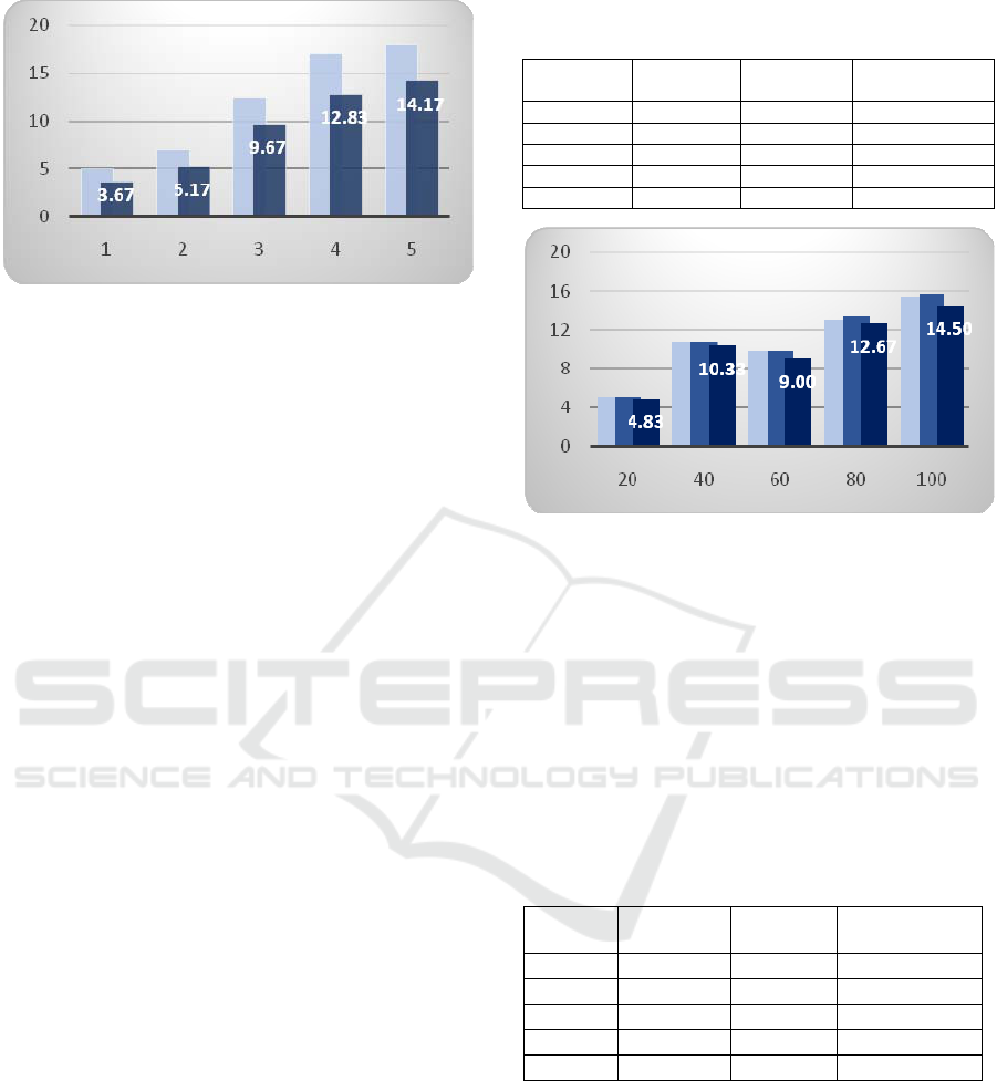
Figure 10: Visualisation of the results for input of type

mixed types (average of used bins) from Table 5. The

original algorithm – light grey and our modified algorithm

– dark grey. X-axis: simulation number (20 to 100 items,

step 20), Y-axis: average number of used bins.

The 4 tables 2, 3, 4, 5 have shown that our

program always outperforms the original program in

all cases. In addition, the 4 figures 7, 8, 9, 10 have

demonstrated that the difference between our

program and the original program increases when

the input size increases. In other words, our program

works better with bigger data set. These results

shown that our program seems to be able to yield

acceptable results for the main experiment in section

5 EXPERIMENTAL RESULTS

This section is the central component of our paper

where experimental results are produced to support

our claim that the order of placement is not relevant

in solving the problem of 2D bin packing. In this

section, the same algorithm described in section 4 is

employed. The algorithm will be run on the same set

of test cases from subsection 4.4, and for each test

case, 3 different orderings will be considered: the

first two orderings will be randomly generated

whilst for the final, it is the area decreasing order,

the results of which have already been available in

subsection 4.4. Our experimental results are

summarized in the following tables and figures.

Table 6, 7, 8 and 9 will summarize our results for

input objects of different types Star, Polygon, Cycle

and Mixed (combination of Star, Polygon and

Cycle), respectively, followed by their

corresponding figures giving an overview of their

data.

Table 6: Average number of bin used for input of type Star

– random orders versus area decreasing order.

Number of

items

Random 1 Random 2

Area

Decreasing

20 5.00 5.00 4.83

40 10.67 10.67 10.33

60 9.83 9.83 9.00

80 13.00 13.33 12.67

100 15.50 15.67 14.50

Figure 11: Visualisation of the results for Star-type items

(average of used bins) form Table 6. The random 1 order –

light grey, random 2 – grey and the area decreasing order

– dark grey. X-axis: Number of items, Y-axis: average

number of used bins.

According to table 6, the program yields the best

results on area decreasing order of input. The

differences range from 0.17 to 1.17 bin. However,

figure 11 shows that their differences are visually

insignificant compared to the number of bins

needed.

Table 7: Average number of bin used for input of type

Polygon – random orders versus area decreasing order.

Number

of items

Random 1 Random 2 Area

Decreasin

7.67 8.00 6.67

16.00 15.33 15.00

22.00 21.83 20.83

15.67 15.83 15.00

100

32.33 32.00 29.83

Table 7 shows that the area decreasing order of

input is still the best ordering. However, as can be

seen from figure 12, there is visually not much

difference when input size is less than 100.

Considerations on 2D-Bin Packing Problem: Is the Order of Placement a Relevant Factor?

285

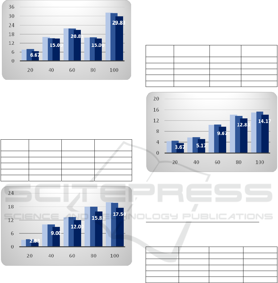
Figure 12: Visualisation of the results for Polygon-type

items (average of used bins) form Table 5. The random 1

order – light grey, random 2 – grey and the area

decreasing order – dark grey. X-axis: Number of items, Y-

axis: average number of used bins.

Table 8: Average number of bin used for input of type

Circle – random orders versus area decreasing order.

Number

of items

Random 1 Random 2

Area

Decreasing

20 3.17 3.33 2.33

40 10.00 10.00 9.00

60 13.17 13.33 12.00

80 18.00 18.00 15.83

100 20.00 19.67 17.50

Figure 13: Visualisation of the results for Circle-type

items (average of used bins) form Table 5. The random 1

order – light grey, random 2 – grey and the area

decreasing order – dark grey. X-axis: Number of items, Y-

axis: average number of used bins.

In table 8, the area decreasing order remains as

the best ordering. Albeit the differences are wider

between the three compared to previous results, they

are at most 2.5 for input size of 100 which is still an

acceptable result considering the height of its

corresponding bar. Figure 13 shows that the three

bars for each input size seem very close in height.

Table 9 shows results for inputs of mixed types

which are the most general case in the experiment.

The area decreasing order is still the best, but closer

analysis on the relationship between the maximum

difference between the three orderings and the best

number of bin used can reveal an interesting pattern.

For each input size, consider the following ratio.

Table 9: Average number of bin used for input of mixed

types – random orders versus area decreasing order.

Number

of items

Random 1 Random 2

Area

Decreasing

20 4.33 4.50 3.67

40 5.67 5.83 5.17

60 10.33 10.50 9.67

80 14.17 13.67 12.83

100 15.00 15.33 14.17

Figure 14: Visualisation of the results for items of mixed

types (average of used bins) form Table 5. The random 1

order – light grey, random 2 – grey and the area

decreasing order – dark grey. X-axis: Number of items, Y-

axis: average number of used bins.

axValueO

Bin –

inValueO

Bin

(1)

inValueO

Bin

Table 10: Results for comparison following formula (1).

Input Size Max Min Ratio (1)

20 4.50 3.67 22.6%

40 5.83 5.17 12.8%

60 10.50 9.67 8.6%

80 14.17 12.83 10.4%

100 15.33 14.17 8.2%

The ratio values tend to decrease as the input size

increases. In other words, the program performs

more similar on different orderings for larger input

size. Even for the small input size like 20, though

the fraction seems high but the real difference is just

0.83 bin. For each input size, all results are still

relatively close as illustrated in figure 14. This

comparison is only made for this input since this is

the most general case where objects are more

diverse in shapes. The other types of input are too

specific and may require more tests of a more

variety of sizes for the pattern to be clearly present.

All results confirm that random orderings are

good since they are not too far away from the area

SIMULTECH 2017 - 7th International Conference on Simulation and Modeling Methodologies, Technologies and Applications

286

decreasing order which has already been known as

an excellent order. In all test cases, the average

difference between the area decreasing order and

random orders never exceeds 2.5 bins for input size

of 100. The 4 figures also show that there is visually

not much difference between them. An important

consideration is that results on the two randomly

generated orderings are almost identical. The

maximum difference between them is 0.67 bin as

shown in table 7 for input size of 40. If the order of

placement is an important factor, there is no possible

way that they do not differ by even 1 bin in all 120

test cases. That implies that all possible orders of

placement should generally yield very close results.

Considering our results and results from

Ferreira

shown in table 1

, we strongly believe that the order of

placement is not relevant for researches in this topic.

Our experimental results do not demonstrate that the

order of placement has no effect at all in this

problem, but they confirm that the influence is so

little that even a random permutation of input should

be good comparatively to the best one. Hence there

is no practical benefit in using complicated

optimization techniques, which should be about

hundreds of times slower than a normal greedy

approach especially for large input size, to find the

best order of placement. Further researches into this

topic should investigate into other dimensions such

as the placement method.

6 CONCLUSION AND FUTURE

WORK

Our study investigates the relevance of the order of

placement, which has been one of the main

objectives of optimization, in the 2D bin packing

problem, and conclude that its influence is so little

that it does not deserve the attention of researchers

in this topic by using experimental results to show

that even random orderings may yield very good

results comparable to a good ordering.

Improvements should be made on the placement

method instead of the order of placement. We

believe an advanced placement method with a

simple order of placement would outperform a

simple method with complicated order of placement.

Even though our experiment yields generally

acceptable results, it is not up to our expectation. We

believe that the differences between the three

orderings in section 5 may be even closer if a better

placement algorithm is used. Our placement

algorithm is acceptable, but it is based on a regular

packing algorithm which is not fully intended for the

irregular problem.

In future experiments, we will continue

investigating into other placement methods that are

designed for the irregular packing problem to

produce better experimental results. In addition, we

would like to make one-to-one comparisons between

random orderings with orderings generated from

advanced search techniques such as Simulated

Annealing or Evolutionary Algorithm to point out

how little the algorithm may improve at the huge

cost of resource consumption.

REFERENCES

Duarte Nuno Gonçalves Ferreira, 2015. Rectangular Bin-

Packing Problem: a computational evaluation of 4

heuristics algorithms. U. Porto Journal of Engineering,

1:1 (2015) 35-49.

Moises Baly, 2016. Java Implementation for 2D Bin

Packing. [Online]. [Accessed on 20 April 2017].

Available from https://github.com/mses-bly/2D-Bin-

Packing.

Alvim, A.C.F., F. Glover, C.C. Ribeiro, and D.J. Aloise.

1999. “Local Search for the Bin Packing Problem.” In

Extended Abstracts of the 3rd Metaheuristics

International Conference, Angra dos Reis, pp. 7-12.

R.L. Rao, S.S. Iyengar, 1994. Bin-Packing by Simulated

Annealing. Computers Math. Applic. Vol. 27, No. 5,

pp. 71-82.

Jordan Junkermeier, 2015. A Genetic Algorithm for the

Bin Packing Problem. Evolutionary Computation, St.

Cloud State University, Spring 2015.

György Dósa, Jiří Sgall, 1998. First-Fit bin packing: A

tight analysis. 1998 ACM Subject Classification F.2.2

Nonnumerical Algorithms and Problems.

A. Lodi, S. Martello, M. Monaci, D. Vigo, 2010. Two-

Dimensional Bin Packing Problems. In Paschis V. Th.

Paradigms of Combinatorial Optimization,

Wiley/ISTE, p. 107-129.

Andrea Lodi, Silvano Martello, Daniele Vigo, 2002.

Recent advances on two-dimensional bin packing

problems. Discrete Applied Mathematics 123 (2002)

379–396.

Bennell, J.A, and Oliveria, J.F, 2008. 50 years of irregular

shape packing problems: a tutorial/ Southampton, UK

(Discussion Papers in Centre for Operational

Research, Management Science and Information

Systems, CORMSIS-08-14).

Jukka Jylänki, 2010. A Thousand Ways to Pack the Bin - A

Practical Approach to Two-Dimensional Rectangle

Bin Packing. [Online]. [Accessed on 20 April 2017].

Available from http://clb.demon.fi/files/RectangleBin

Pack.pdf.

Joseph O'Rourke, 1985. Finding minimal enclosing boxes.

International Journal of Computer & Information

Sciences June 1985, Volume 14, Issue 3, pp 183–199.

Considerations on 2D-Bin Packing Problem: Is the Order of Placement a Relevant Factor?

287