A Novel Approach for Handling Discontinuities in Non-iterative
Co-simulation
Daniela Dejaco and Martin Benedikt
VIRTUAL VEHICLE Research Center, Inffeldgasse 21A, Graz, Austria
Keywords:
Distributed Hybrid Systems, Weak Coupling, Co-simulation.
Abstract:
In this work, a novel approach for the co-simulation of systems with discontinuities is presented. Currently,
an extensive literature exists on the simulation of distributed systems as well as on the proper discontinuity
handling during simulation. The not trivial task is to design a simulation platform that is able to do both at the
same time.
The proposed algorithm, which extends an existing non-iterative co-simulation strategy, administrates the
mutual communication between two subsystems to assure that events are propagated correctly within the
distributed system. Based on a prediction of future event triggering, the co-simulation sequence is chosen and
thus the discontinuities are handled with no need of “rolling-back” or of iterating.
A simulation example demonstrates the efficiency of the outlined algorithm.
1 INTRODUCTION
A hybrid system is a dynamic system where a contin-
uous time behavior is combined with a discrete time
behavior. This means that the system is both capable
of flowing and of jumping. The continuous character
of the system is described by a differential equation,
while the discrete time part is modeled by an automa-
ton. Hence, the current state of the overall system is
described by both the continuous state x(t) and the
current discrete mode (Henzinger, 1996).
The jumps between the various modes of the system
are associated to so called “events”. We distinguish
between two types of events:
• Time events, triggered at a previously known
time;
• State events, triggered if a condition associated to
the continuous state x(t) is satisfied, i. e. if the
continuous state x(t) reaches a certain threshold.
The time-discretization paradigm for simulating
physical systems is nowadays a well known and es-
tablished field of studies; its origins can be attributed
to the deeper studies of system theory (see for exam-
ple (Zadeh and Desoer, 1963)). For this simulation
paradigm, the simulation of time events is straightfor-
ward. The simulation across state events is a bit more
challenging, because whenever the solution crosses
through a state event, the exact time instant of the
discontinuity must be detected. For real-time simu-
lation, interpolation methods of low order are prefer-
able, while for a more accurate detection of the ex-
act event time iterative methods are applied (Cellier
and Kofman, 2006). Although there is a huge variety
of methods for both discontinuity detection and exact
event localization (see for example (Park and Barton,
1996) or (Zhang et al., 2008)), no current method can
guarantee the proper functioning for all possible sys-
tems to be simulated. Hence, the task is to find the
method that applies best to the specific use case.
A more recently developed numerical simulation
strategy, termed Quantized State Simulation (QSS)
(Cellier and Kofman, 2006) (Cellier et al., 2008), pro-
poses to discretize the state valuesinstead of discretiz-
ing the time. While the time-discretization algorithms
convert Ordinary Differential Equation (ODE) sys-
tems to equivalent difference equation systems, the
QSS algorithms convert the continuous-time model
to an equivalent discrete-event model. The obtained
discrete-event model can then be simulated using
a discrete-event simulation engine, for example the
Discrete Event System Specification (DEVS) (Zei-
gler et al., 2000). The asynchronous nature of this
algorithm makes it a very powerful method for state
event handling; detecting if the continuous state x(t)
reaches a threshold is exactly what QSS algorithms
are designed for. Hence, as no iteration is needed at
discontinuities, it is well suited for real-time simula-
288
Dejaco, D. and Benedikt, M.
A Novel Approach for Handling Discontinuities in Non-iterative Co-simulation.
DOI: 10.5220/0006440402880295
In Proceedings of the 7th International Conference on Simulation and Modeling Methodologies, Technologies and Applications (SIMULTECH 2017), pages 288-295
ISBN: 978-989-758-265-3
Copyright © 2017 by SCITEPRESS – Science and Technology Publications, Lda. All rights reserved

tion. However, only for QSS of first order the event
localization is exact; for higher orders, the localiza-
tion is based on a linearization of the derivatives at
the current point (Cellier et al., 2008).
The numerical simulation problem gets more intricate
if the system to be simulated is a large-scaled cyber-
physical system (CPS). Due to the increased complex-
ity, the hybrid character and the different areas of en-
gineering covered, it is typically necessary to split the
overall system in separated subsystems. Each sub-
system is modeled withing a specific domain and is
solved separately by a tailored solver. An efficient
coupling of these subsystems is thus necessary in or-
der to simulate the CPS properly. A commonly used
methodology is the so called co-simulation, where
each subsystem is solved independently over a cer-
tain time interval (macro-step), at the end of which the
subsystems are allowed to exchange information. For
this purpose, the functional mockup-interface (FMI)
(Blochwitz et al., 2012) for Co-simulation was estab-
lished as a tool independent standard to support the
exchange and the (protected) integration of various
subsystems even if different simulation tools are used.
In terms of co-simulation, iterative and non-iterative
numerical schemes are available for adequate sub-
system integration. Iterative approaches strictly re-
quire resetting of subsystems (and of their solvers)
and can therefore be applied only to a very limited set
of tools. On the other hand, non-iterative approaches
state marginal requirements on simulation tools and
can be applied in general. In case of closed loops, es-
timation of the future output of dedicated subsystems
is performed by extrapolation.
The main idea is to estimate the future output of a sub-
system by extrapolation. This estimation is then used
as an input to simulate the subsequent subsystem over
the next macro-step.
This co-simulation strategy is termed weak coupling,
as each subsystem can be treated as a black-box and
no information about its internal structure is needed
for co-simulation purposes.
Up to date, co-simulation platforms, as well as the
“FMI for Co-Simulation” 2.0 (Blochwitz et al., 2012),
is currently focusing on continuous system simula-
tion, limiting simulation accuracy. The purpose of
this work is to propose a solution of how non-iterative
co-simulation can be extended in order to be able to
simulate properly hybrid systems.
The aforementioned QSS simulation paradigm can
easily be extended to the simulation of distributed sys-
tems (Bergero et al., 2013). As previously mentioned,
the QSS converts the various subsystems to discrete-
event models. In literature, there are quite a lot of so-
lutions for the simulation of distributed discrete-event
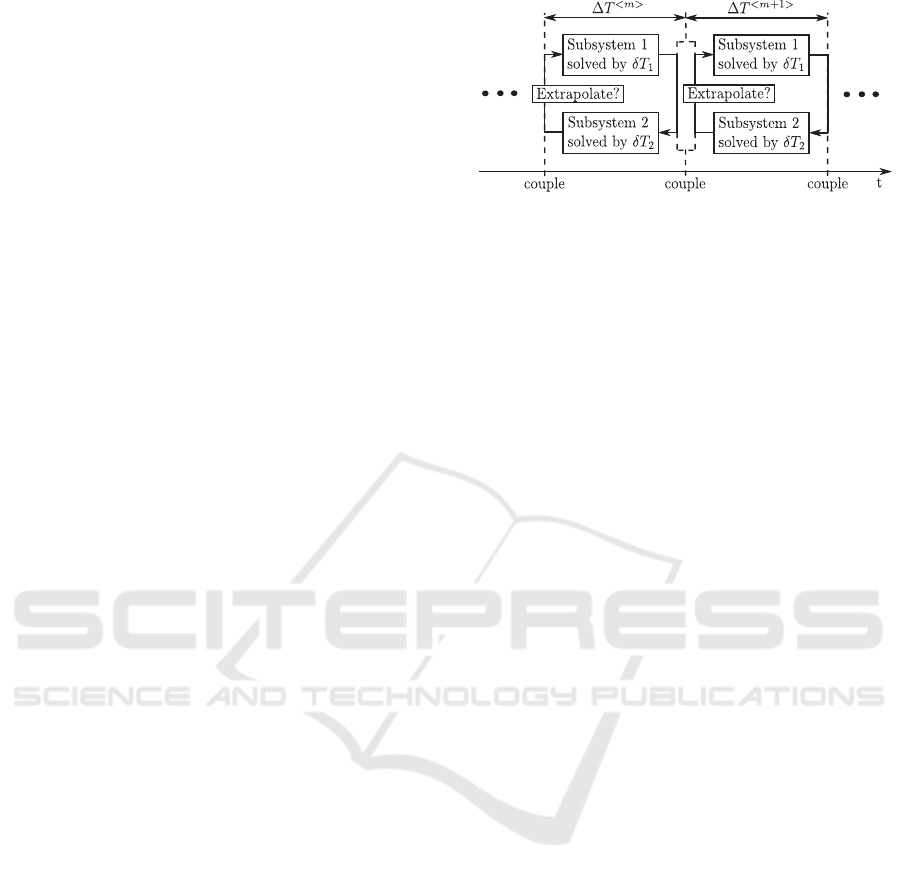
Figure 1: Principle of the sequential, non-iterative co-
simulation approach.
models. In general they can be categorized into so
called optimistic approaches (see for example (Jeffer-
son, 1985)) and conservative approaches (see for ex-
ample (Chandy and Misra, 1979)).
Besides the lower accuracy in comparison to the well
known time-discretization simulation, the biggest
drawback of applying QSS to co-simulation is that
most of the co-simulation platforms and integrated
tools are currently designed for numerical simulation
with time-discretization.
In this work, a novel approach of non-iterative co-
simulation of hybrid systems is proposed. The non-
iterative and time-discretizing nature will be pre-
served, but some additional knowledge of the in-
ternal structure of the models is needed. How-
ever, only slight modifications on the FMI standard
would be necessary. The need of adapting the FMI
standard to hybrid systems is currently discussed in
the FMI working group “Clocks and Hybrid Co-
Simulation”(Broman et al., 2015).
Section 2 is devoted to non-iterative co-simulation
and presents a simple hybrid system. Furthermore,
extensions of common non-iterativeco-simulation ap-
proaches are briefly discussed. In Section 3, the pro-
posed algorithm is exposed. The algorithm is then
applied and the results are discussed in Section 4. Fi-
nally, in Section 5 two important extensions to the al-
gorithm are proposed.
2 PROBLEM DESCRIPTION
2.1 Non-iterative Co-simulation
Most integration platforms use a non-iterative cou-
pling approach to co-simulate distributed systems.
Each subsystem is solved independently using a suit-
able fixed or a variable micro-step δT. At predefined
points in time, the simulations are paused and data
can be exchanged between the subsystems. The time
intervals between these points are termed macro-steps
∆T. As shown in Figure 1, in order to solve the
A Novel Approach for Handling Discontinuities in Non-iterative Co-simulation
289

closed loops in the distributed networks, the output of
subsystem 2 is extrapolated (based on the history of
simulation data) and fed into subsystem 1. Subsystem
1 can then be simulated over the macro-step and its
output allows to simulate subsystem 2. The choice of
the scheduling, the order of extrapolation as well as
of the macro-step size is crucial and is discussed in
(Benedikt et al., 2013a).
In this example, the subsystems within the co-
simulation are scheduled in sequential order, i.e.
the subsystems are not simulated in parallel. Of
course, this is more time consuming in general, but
significantly increases accuracy as well as numerical
stability. For real-time applications, at the price of
decreasing accuracy, it is possible to extrapolate the
outputs of both subsystems and hence simulate the
subsystems in parallel.
A recently proposed extension to the classical
non-iterative co-simulation scheme, called NEPCE
(Benedikt and Hofer, 2013), estimates the error com-
mitted by extrapolation for the current macro-step
and compensates it during the subsequent steps in
terms of energy preservation.
This approach is extended for application of smooth-
ing filters, effectively reducing aliasing effects. In
(Drenth, 2016) the benefit of filtering techniques is
demonstrated along very stiff system integration. Re-
cently, in (Sadjina and Pedersen, 2016), an extension
of NEPCE for incorporation of direct feedthrough
was done. For handling stiff systems linearly-implicit
schemes are proposed (Arnold et al., 2007).
However, these mechanisms are not adequate to
simulate distributed systems with discontinuities
described by state events. An extension to the non-
iterative approach that is able to do so is proposed in
this paper.
Note: For the proposed algorithm to work, it is
mandatory that the solvers of each subsystem are
capable of simulating across discontinuities.
2.2 A Simple Example
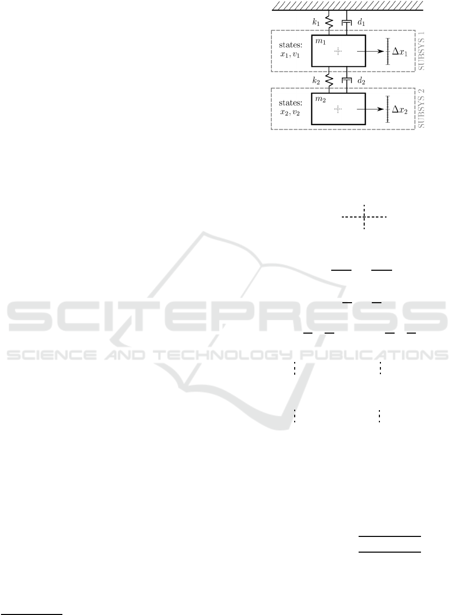
The hybrid system on which the algorithm is tested is
shown in Figure 2. It consists of a mass m
1
connected
to the ceiling by a spring and a damper with coef-
ficients k
1
and d
1
, respectively. Similarly, a second
mass m
2
is connected to the first mass by a spring-
damper element with coefficients k
2
and d
2
. Let x
i
(t)
and v
i
(t) be the position and velocity, respectively, of
the mass i with respect to the ceiling.
1
The continuous
time behavior of the hybrid system can then be de-
1
For the sake of simplicity, the time t will be omitted
from now on
Figure 2: Test case: two-mass-spring-damper system con-
nected to the ceiling. The system is split into two subsys-
tems, each one corresponding to a single mass and its posi-
tion and velocity as state variables.
scribed by the following set of differential equations:
˙
z = Az+ g =

A
1
B
1
B
2
A
2

z+ g, (1)
where the matrix A is composed of
A
1
=

0 1
−
k
1
+k
2
m
1
−
d
1
+d
2
m
1

, (2)
A
2
=

0 1
−
k
2
m
2
−
d
2
m
2

, (3)
B
1
=

0 0
k
2
m
1
d
2
m
1

,B
2
=

0 0
k
2
m
2
d
2
m
2

(4)
and the vector g is given by
g =

g
T
1
g
T
2

T
=

0 −g 0 −g

T
, (5)
with g being the gravitational acceleration. The state
space vector of the overall system is:
z =

z
T
1
z
T
2

T
=

x
1
v
1
x
2
v
2

T
. (6)
This hybrid system is composed of only one mode,
but there are two events that can cause a discontinuity
in the state vector:
• The mass m
1
hits the ceiling
IF (x
1
≥ −∆x) & (v
1
≥ 0)
RESET v
1,new
= −v
1
• The two masses collide
IF ((x
1
− x
2
) ≤ 2∆x) & ((v
1
− v
2
) ≤ 0)
RESET

v
1,new
v
2,new

=
"
(m
1
+m
2
)v
1
+2m
2
v
2
m
1
+m
2
(m
1
+m
2
)v
2
+2m
1
v
1
m
1
+m
2
#
As shown in Figure 2, the overall system is split
into two subsystems, each one corresponding to one
of the two masses.
Thus, the continuous time dynamics of subsystem 1
are described by
˙
z
1
= A
1
z
1
+ B
1
u
1
+ g
1
, (7)
SIMULTECH 2017 - 7th International Conference on Simulation and Modeling Methodologies, Technologies and Applications
290

where the input u
1
corresponds to the state vector of
subsystem 2:
u
1
=

u
1x
u
1v

= z
2
. (8)
Similarly, the continuous time dynamics of subsystem
2 can be written as
˙
z
2
= A
2
z
2
+ B
2
u
2
+ g
2
, (9)
with input
u
2
=

u
2x
u
2v

= z
1
. (10)
But what about the state events that cause the jumps in
the state variables? We can clearly see that the condi-
tion corresponding to the mass m
1
hitting the ceiling
only depends on the state variables of subsystem 1.
Even the jump in the state variables only affects this
subsystem. Hence, this event will be termed Private
state event.
The state event corresponding to the collision of the
two masses, instead, depends on the state variables of
both subsystems and the reset condition affects both.
Thus, these events will be referred to as Shared state
events.
The discontinuities of subsystem 1 can thus be written
as:
• Private State Event: The mass m
1
hits the ceiling
IF (x
1
≥ −∆x) & (v
1
≥ 0)
RESET v
1,new
= −v
1
• Shared state event: The two masses collide
IF ((x
1
− u
1x
) ≤ 2∆x) & ((v
1
− u
1v
) ≤ 0)
RESET v
1,new
=
(m
1
+m
2
)v
1
+2m
2
u
1v
m
1
+m
2
while the only event that can be triggered in subsys-
tem 2 is:
• Shared State Event: The two masses collide
IF ((u
2x
− x
2
) ≤ 2∆x) & ((u
2v
− v
2
) ≤ 0)
RESET v
2,new
=
(m
1
+m
2
)v
2
+2m
1
u
2v
m
1
+m
2
.
In order for the proposed algorithm to work, there
must exist a link between the shared state events of
the two subsystems. In an object-oriented program-
ming paradigm, for example, the events can be treated
as objects and include a pointer to the correspond-
ing event in the other subsystem. Due to this nec-
essary change, the subsystems can no longer be seen
as “black boxes” as it is state-of-the-art in common
co-simulation platforms.
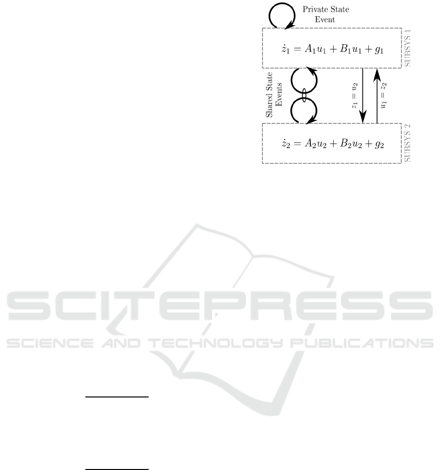
Figure 3 summarizes the hybrid behavior of both sub-
systems and shows the necessary links between the
two subsystems.
Figure 3: Continuous and discrete-event dynamics of both
subsystems. The continuous time dynamics of the two
subsystems are connected by an algebraic loop, while the
shared state events must contain a link to each other.
2.3 Necessary Extensions
A significant problem arises when a shared event is
triggered only in one of the two subsystems. In our
test case this means that for example the upper mass
changes direction due to a collision with the lower
mass, while the lower mass does not recognize the
occurrence of the event. This violates the laws of
physics.
Alternatively, it can happen that a shared event is trig-
gered in subsystem 1 and the reset on the state vari-
ables is done accordingly. If the same shared event is
triggered in subsystem 2 with a small delay, the reset
of the state variables proves to be completely wrong.
As stated, the reset condition depends on u
2
= z
1
. For
a correct implementation, the reset condition should
be calculated based on z
1
before its jump; in this case,
however, due to the small delay, the reset of subsys-
tem 2 is calculated after the jump in subsystem 1.
Finally, private state events cause abrupt changes in
the state variables of one subsystem. This jump prop-
agates to the second subsystem according to its ordi-
nary differential equation. If no changes are applied
to the co-simulation paradigm, however, the informa-
tion about the jump is sent only after the end of the
macro-step. This delay in the loop can cause oscilla-
tions.
In order to avoid these unpredictable errors, an algo-
rithm for the correct co-simulation of hybrid systems
is proposed in the following section.
A Novel Approach for Handling Discontinuities in Non-iterative Co-simulation
291

3 ALGORITHM
3.1 Requirements and Main Idea
Summarizing, the requirements on the co-simulation
platform to apply the proposed algorithms are:
• Each subsystem must be capable of simulating
across discontinuities. That means that it must be
able to detect discontinuities and it must be able
to locate them accurately either by interpolation
or by iteration.
• There must be a (bilateral) link from a shared state
event to its corresponding shared state event in the
other subsystem.
• Each subsystem must be capable of interrupting
its own simulation even within a macro-step. Af-
ter such an interruption it can notify this occur-
rence to the co-simulation platform. Note that it
is not demanded that a subsystem be able to stop
the simulation of the other subsystem, but merely
to interrupt its own simulation procedure.
The proposed algorithm is designed for sequential
co-simulation and cannot be completely extended to
a parallel paradigm. In section 5, however, it is
briefly discussed how the algorithm could be re-
designed to switch between a sequential and parallel
co-simulation mechanism.
The main idea behind the algorithm is that, as soon
as an event is detected in one subsystem, the simula-
tion should be stopped and the occurrence of the event
should be notified to the other subsystem. As one sub-
system is only capable of stopping its own simulation
and as it is not possible to “roll back”, the first sys-
tem to be simulated must be the one where a private
state event is more likely to occur within the next step.
If the event is a shared state event, instead, after in-
terrupting the simulation of the first subsystem, the
exact event time must be notified to the second sub-
system. Furthermore, the bilateral links between the
shared state events serve to communicate to the sec-
ond subsystem which event was triggered.
For our test case, the upper mass (subsystem 1) is
the only one where private state events are possible,
hence the co-simulation sequence will be, for each
macro-step ∆T:
1. Extrapolate subsystem 2
2. Simulate subsystem 1
3. Simulate subsystem 2.
In section 5 it will be shown how the simulation se-
quence is chosen at the beginning of each macro-step
if it is not trivial.
3.2 Detailed Description
Having chosen a proper co-simulation sequence, a
suitable macro-step ∆T and interruption time εT (see
subsection 3.2.1), the algorithm can be written in de-
tail as follows.
For each macro-step ∆T:
I EXTRAPOLATE SUBSYSTEM 2: The output
of subsystem 2 is extrapolated with a polynomial
of first order (zero-order for the first iteration).
II SIMULATE SUBSYSTEM 1: Using the ex-
trapolated output of subsystem 2 as an input, sub-
system 1 should be simulated till the next macro-
step point, unless an event is detected within the
current step, i.e.:
• If a private state event is detected at time t
e
,
the simulation should be interrupted at t
stop
=
t
e
+ εT
• If a shared state event is detected at time t
e
,
a link to its co-event e should be created and
the simulation should be interrupted at t
stop
=
t
e
+ εT
It is necessary to extend the simulation by a small
time lap εT to assure that there are at least two
samples available if an extrapolationof first order
is demanded.
III SIMULATE SUBSYSTEM 2:
• If the simulation of subsystem 1 was not in-
terrupted by any event, simulate subsystem 2
without allowing it to trigger events.
• If the interruption in subsystem 1 was due to
a private state event, simulate subsystem 2 till
t
e
, and then simulate it till t
stop
.
• If the interruption in subsystem 1 was due to
a shared state event, simulate subsystem 2 till
t
e
, trigger event e and continue simulation till
t
stop
.
IV CHECK: The state vector of both subsystems
must now be visible within the co-simulation
platform. In very rare cases it can happen that:
• A private state event in subsystem 1 was not
detected during the simulation, but is detected
now. In that case trigger the event in subsys-
tem 1.
• A shared state event was not triggeredproperly
and is recognized now. Trigger the event in
both subsystems.
• Due to a wrong setting in the simulation se-
quence a private state event is recognized in
subsystem 2; trigger the event now.
SIMULTECH 2017 - 7th International Conference on Simulation and Modeling Methodologies, Technologies and Applications
292

After having triggered the event, extrapolate sub-
system 2, simulate subsystem 1 till t
∗
stop
= t
stop
+
εT and then simulate subsystem 2 till t
∗
stop
. No
event triggering is allowed in none of the systems
during this short time εT; if a state event is de-
tected, don’t trigger it, but repeat step CHECK.
V ITERATE: Go back to I unless simulation time
is over.
3.2.1 Choice of Interruption Time εT
The interruption time εT must be chosen small
enough to ensure that no two consecutive events hap-
pen within this time. Obviously, zeno-chattering phe-
nomena, which cannot be simulated properly nei-
ther in a mono-simulation, cannot be handled in
the co-simulation paradigm (Lunze and Lamnabhi-
Lagarrigue, 2009). Furthermore, εT must be at least
as large as the minimum step-size in each internal
solver and must be large enough to avoid discontinu-
ity sticking (Park and Barton, 1996).
4 SIMULATION EXAMPLE
To demonstrate the efficiency of the proposed algo-
rithm, it is tested on the mass-damper system de-
scribed in 2.2. The results of the co-simulation are
then compared to a mono-simulation, i.e. where the
overall system is simulated within a single solver. Ne-
glecting numerical errors, we can assume that the re-
sults of the mono-simulation are correct.
To simulate the dynamic behavior of the system, for
both co-simulation and mono-simulation, a Runge-
Kutta-algorithm of 4th order is used. If a disconti-
nuity is detected, it is located accurately using a bi-
section algorithm.
The physical parameters used for the simulation are
m
1
= 0.2kg, m
2
= 0.3kg, d
1
= d
2
= 0.01kg/ s, k
1
=
k
2
= 1kg/s
2
and ∆x = 0.55m, while the initial values
are set:

x
1
v
1

(t=0)
=

−0.7
3.5

,

x
2
v
2

(t=0)
=

−8.8
3

.
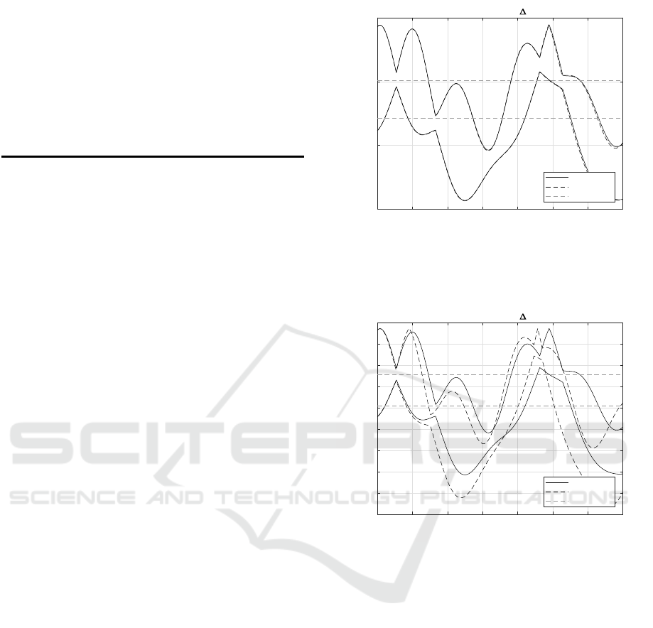
Figure 4 shows the simulation results using a
macro-step size of ∆T = 0.1s and an interruption time
of εT = 10
−4
. We can see that even for a quite
long macro-step, the algorithm performs very well as
the trends of co-simulation and mono-simulation are
identical.
0 1 2 3 4 5 6 7
Time in [s]
-15
-10
-5
0
Height in [m]
Co-Simulation with T = 0.1s
x SIM
x COSIM
stability points
Figure 4: Co-simulation vs. mono-simulation of the test
case described in 2.2. The graphic shows only the state vari-
ables describing the positions x
1
and x
2
of the two masses.
Macro-step ∆T = 0.1s. The results are good.
0 1 2 3 4 5 6 7
Time in [s]
-18
-16
-14
-12
-10
-8
-6
-4
-2
0
Height in [m]
Co-Simulation with T = 0.3s
x SIM
x COSIM
stability points
Figure 5: Co-simulation vs. mono-simulation of the test
case described in 2.2. The graphic shows only the state vari-
ables describing the positions x
1
and x
2
of the two masses.
Macro-step ∆T = 0.3s. At t = 0.9s, in the co-simulation,
a wrong event is detected which leads to unpredictable re-
sults.
In contrary, using the macro-step ∆T = 0.3s, the co-
simulation for hybrid system does not give good re-
sults for this test case. In Figure 5, we can clearly see
that at t = 0.9s, a private state event (The mass m
1
hits
the ceiling) is detected in the co-simulation, whilst
this is not the case in the mono-simulation. This event
error is then propagated throughout the simulation
and leads to totally wrong and unpredictable results.
Although these two examples show that the choice of
the macro-step size is crucial for the co-simulation,
it is shown in (Benedikt et al., 2013b) how NEPCE
could significantly improve the simulation even for
larger macro-steps.
A Novel Approach for Handling Discontinuities in Non-iterative Co-simulation
293

5 EXTENSIONS
5.1 Automatic Co-simulation Sequence
As previously explained, for the test case the co-
simulation sequence is trivial. Only subsystem 1 trig-
gers private state events and is hence the subsystem to
be simulated first.
If both subsystems can trigger private state events, the
co-simulation sequence must be set at the beginning
of each macro-step. The setting is based on a predic-
tion of which subsystem is more likely to trigger a pri-
vate event withing the next macro-step. The proposed
procedure is likely to work properly, but in some very
rare cases it can fail. If it fails, however, it will be rec-
ognized with a small delay during the CHECK phase
in the algorithm proposed in 3.2.
For the first iteration, the co-simulation sequence
must be set randomly. For the following itera-
tions the technique is the following (the assump-
tion is that currently subsystem 1 is simulated first):
• Set ∆T
∗
= 1.5∆T.
• Extrapolate subsystem 2 till ∆T
∗
and check if a
private event is triggered.
• IF no private event is triggered, keep the co-
simulation sequence.
• IF a private event is triggered, extrapolate subsys-
tem 1 till ∆T
∗
and check if a private event is trig-
gered.
– IF no private event is triggered in subsystem 1,
switch the simulation sequence.
– IF a private event is triggered in subsystem 1,
do some iterations to find out which subsys-
tem is supposed to trigger its private event first.
This subsystem is the subsystem to be simu-
lated first.
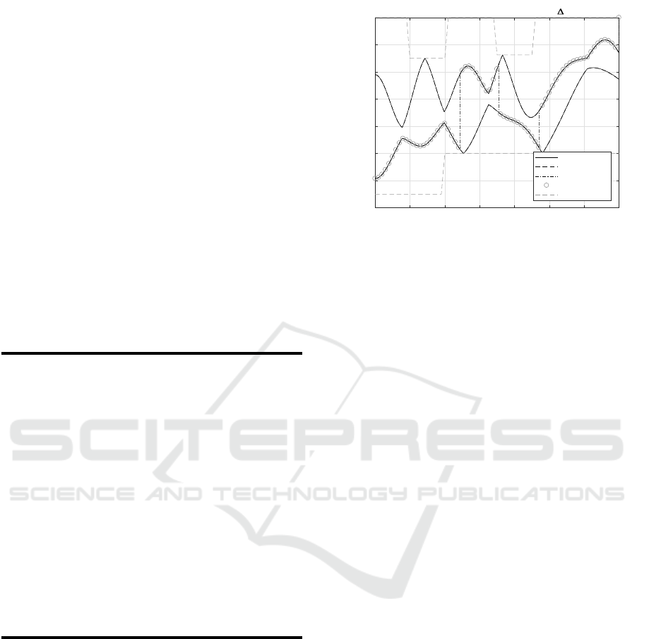
To prove the correctness of this idea, a co-simulation
example is shown in Figure 6. It referres to the usual
test case, but in this case the ceiling is not standing
still anymore. In addition, the mass m
2
can hit the
floor, which is moving as well. This means that both
subsystems are capable of jumping due to a private
state event.
Here, the gray dashed lines show the extrapolated
outputs that are used for co-simulation purposes. We
can see that till t = 2.4s subsystem 2 is extrapolated
(default co-simulation sequence). At t = 2.4s, the
co-simulation sequence is switched because a private
state event in subsystem 2 is predicted. The sequence
is switched again at t = 3.55s and at t = 4.75s.
0 1 2 3 4 5 6 7
Time in [s]
-14
-12
-10
-8
-6
-4
-2
0
Height in [m]
Co-simulation with automatic sequence. T = 0.05
x SIM
x COSIM
switch sequence
x EXTRAP
floor and ceiling
Figure 6: Co-simulation vs. mono-simulation for the test
case extended to both subsystems capable of performing
private state events. The graphic shows only the state vari-
ables describing the positions x
1
and x
2
of the two masses.
Macro-step ∆T = 0.05s.
5.2 Parallel Co-simulation
Due to real-time requirements, in many applications it
is preferable to simulate the two subsystems in paral-
lel. In dynamical systems without discontinuities, the
simple procedure is:
1. Extrapolate both subsystems in parallel
2. Simulate both subsystems in parallel
This strategy is less time-consuming, but even less
precise.
It is not possible to extend the proposed algorithm to
work in parallel for all iterations, but with a similar
approach as in 5.1, it can be predicted if any kind of
discontinuity is likely to occur within the next macro-
step. If it is stated that no event will occur, we can
switch to parallel co-simulation for the next macro-
step.
6 CONCLUSION
In this work, an approach for handling discontinu-
ities in sequential non-iterative co-simulation was ad-
dressed. Currently, most of the co-simulation plat-
forms focus on continuous dynamic systems and ex-
perience various problems if abrupt changes in the
state variables occur. Thus, the developed algorithm
aims to administrate the communication between two
subsystems in order to handle discontinuities prop-
erly. It was stated in the paper that first of all, the co-
simulation sequence is crucial, i.e. which of the two
subsystems is to be simulated first. During the simu-
lation of the first subsystem, the simulation has to be
SIMULTECH 2017 - 7th International Conference on Simulation and Modeling Methodologies, Technologies and Applications
294

stopped as soon as an event occurs and the event must
be communicated to the second subsystem. In order
to apply the proposed algorithm, slight changes to the
Functional Mock-Up Interface are demanded, but the
non-iterative character of the co-simulation platform
will be preserved. Finally, it was shown with a simple
simulation example that, provided suitable settings,
the approach leads to accurate simulation results.
ACKNOWLEDGEMENTS
This work was accomplished at the VIRTUAL VE-
HICLE Research Center in Graz, Austria. The au-
thors would like to acknowledge the financial sup-
port of the COMET K2 - Competence Centers for
Excellent Technologies Programme of the Austrian
Federal Ministry for Transport, Innovation and Tech-
nology (bmvit), the Austrian Federal Ministry of Sci-
ence, Research and Economy (bmwfw), the Austrian
Research Promotion Agency (FFG), the Province of
Styria and the Styrian Business Promotion Agency
(SFG).
REFERENCES
Arnold, M., Burgermeister, B., and Eichberger, A. (2007).
Linearly implicit time integration methods in real-
time applications: Daes and stiff odes. Multibody Sys-
tem Dynamics, 17(2):99–117.
Benedikt, M. and Hofer, A. (2013). Guidelines for the ap-
plication of a coupling method for non-iterative co-
simulation. In 8th EUROSIM Congress on Modelling
and Simulation.
Benedikt, M., Watzenig, D., and Hofer, A. (2013a). Mod-
elling and analysis of the non-iterative coupling pro-
cess for co-simulation. Mathematical and Computer
Modelling of Dynamical Systems, 19(5):451–470.
Benedikt, M., Watzenig, D., Zehetner, J., and Hofer, A.
(2013b). Nepce - a nearly energy-preseving cou-
pling element for weak-coupled problems and co-
simulation. In V International Conference on Com-
putational Methods for Coupled Problems in Science
and Engineering.
Bergero, F., Kofman, E., and Cellier, F. E. (2013). A novel
parallelization technique for devs simulation of con-
tinuous and hybrid systems. Simulation, 89(6):663–
683.
Blochwitz, T., Akesson, M. O. J., Arnold, M., Clau, C.,
Elmqvist, H., Friedrich, M., Junghanns, A., Mauss, J.,
Neumerkel, D., Olsson, H., and Viel, A. (2012). Func-
tional mockup interface 2.0: The standard for tool in-
dependent exchange of simulation models. In 9th In-
ternational Modelica Conference.
Broman, D., Greenberg, L., Lee, E. A., Masin, M., Tri-
pakins, S., and Wetter, M. (2015). Requirements for
hybrid cosimulation. In 18th International Conference
on Hybrid Systems: Computation and Control (HSCC
2015).
Cellier, F. E. and Kofman, E. (2006). Continuous System
Simulation. Springer.
Cellier, F. E., Kofman, E., Migoni, G., and Bortolotto, M.
(2008). Quantized state system simulation. In Grand
Challenges in Modeling and Simulation part of SCSC
2008, Summer Computer Simulation Conference, Ed-
inburgh, Scotland.
Chandy, K. and Misra, J. (1979). Distributed simulation:
A case study in design and verification of distributed
programs. IEEE Transactions on Software Engineer-
ing, 5(5):440–452.
Drenth, E. (2016). Robust co-simulation methodology of
physical systems. In 9th Graz Symposium VIRTUAL
VEHICLE.
Henzinger, T. A. (1996). The theory of hybrid automata.
LICS1996: Proceedings of the 11th Annual IEEE
Symposium on Logic in Computer Science.
Jefferson, D. R. (1985). Virtual time. ACM Trans. Program.
Lang. Syst., 7:404–425.
Lunze, J. and Lamnabhi-Lagarrigue, F. (2009). Handbook
of Hybrid Systems Control. Cambridge.
Park, T. and Barton, P. I. (1996). State event location in
differential-algebraic models. In ACM Transactions
on Modeling and Computer Simulation.
Sadjina, S. and Pedersen, E. (2016). Energy conserva-
tion and coupling error reduction in non-iterative co-
simulations. Cornell University Library.
Zadeh, L. A. and Desoer, C. A. (1963). Linear System The-
ory: The State Space Approach. McGraw Hill.
Zeigler, B., Kim, T., and Praehofer, H. (2000). Theory of
Modelling and Simulation. Academic Press.
Zhang, F., Yeddenapudi, M., and Mosterman, P. J. (2008).
Zero-crossing location and detection algorithms for
hybrid systems simulation. In Proceedings of the 17th
World Congress The International Federation of Au-
tomatic Control.
A Novel Approach for Handling Discontinuities in Non-iterative Co-simulation
295