Analysing Dynamical Systems

Towards Computing Complete Lyapunov Functions

Carlos Arg

aez

, Peter Giesl

and Sigurdur Hafstein

Faculty of Physical Sciences, University of Iceland, 107 Reykjav

ık, Iceland

Department of Mathematics, University of Sussex, Falmer BN1 9QH, U.K.

Keywords:

Dynamical System, Complete Lyapunov Function, Meshless Collocation, Radial Basis Functions.

Abstract:

Ordinary differential equations arise in a variety of applications, including e.g. climate systems, and can ex-

hibit complicated dynamical behaviour. Complete Lyapunov functions can capture this behaviour by dividing

the phase space into the chain-recurrent set, determining the long-time behaviour, and the transient part, where

solutions pass through. In this paper, we present an algorithm to construct complete Lyapunov functions. It is

based on mesh-free numerical approximation and uses the failure of convergence in certain areas to determine

the chain-recurrent set. The algorithm is applied to three examples and is able to determine attractors and

repellers, including periodic orbits and homoclinic orbits.

1 INTRODUCTION

In this paper, we describe a new algorithm to analyse

the behaviour of a dynamical system. Let us consider

a general autonomous ordinary differential equation

(ODE)

x = f(x), where x ∈ R

A classical (strict) Lyapunov function (Lyapunov,

1992) is a scalar-valued function that can be used to

analyse the basin of attraction of one attractor such as

an equilibrium or a periodic orbit. It attains its mini-

mum at the attractor, and is otherwise strictly decreas-

ing along solutions of the ODE.

A generalization of this idea is the notion of a

complete Lyapunov function (Conley, 1978a; Con-

ley, 1988; Hurley, 1995; Hurley, 1998), which charac-

terizes the complete behaviour of the dynamical sys-

tem. It is a scalar-valued function V : R

→ R, de-

ﬁned on the whole phase space, not just in a neighbor-

hood of one particular attractor. It is non-increasing

along solutions of the ODE. The phase space can be

divided into the area where the complete Lyapunov

function strictly decreases along solution trajectories

and the one where it is constant along solution trajec-

tories. The area where the complete Lyapunov func-

tion is strictly decreasing along solution trajectories

characterizes the gradient-like ﬂow. There solutions

pass through and the larger this area is, the more in-

formation is obtained from the complete Lyapunov

function. Note that, by deﬁnition, the complete Lya-

punov function needs to be constant along solution

trajectories on each transitive component of the chain-

recurrent set.

Note that there are other methods to analyse the

general behaviour of dynamical systems: The di-

rect simulation of solutions with many different ini-

tial conditions, however, is costly and can only give

limited information about the general behaviour of

the system, unless estimates are available, e.g. when

shadowing solutions. More sophisticated methods in-

clude the computation of invariant manifolds, form-

ing the boundaries of basins of attraction of attractors

(Krauskopf et al., 2005); here, additional analysis of

the parts with gradient-like ﬂow is necessary. The cell

mapping approach (Hsu, 1987) or set oriented meth-

ods (Dellnitz and Junge, 2002) divide the phase space

into cells and compute the dynamics between these

cells, see also for example (Osipenko, 2007); these

ideas have also been used to compute complete Lya-

punov functions, see Section 2.1.

In this paper we focus on a new algorithm of tack-

ling a mathematical problem numerically. Inspired

by a method to compute classical Lyapunov functions

for an equilibrium, we approximate the solution of

(x) = −1, where V

(x) = ∇V (x) · f(x) denotes the

orbital derivative, the derivative along solutions of the

ODE. We use mesh-free collocation with Radial Basis

Function to approximately solve this partial differen-

tial equation (PDE): we choose a ﬁnite set of collo-

cation points X and compute an approximation v to V

which solves the PDE in all collocation points.

134

Argáez, C., Hafstein, S. and Giesl, P.

Analysing Dynamical Systems - Towards Computing Complete Lyapunov Functions.

DOI: 10.5220/0006440601340144

In Proceedings of the 7th International Conference on Simulation and Modeling Methodologies, Technologies and Applications (SIMULTECH 2017), pages 134-144

ISBN: 978-989-758-265-3

Note, however, that the PDE cannot be fulﬁlled

at all points of the chain-recurrent set, such as an

equilibrium or periodic orbit. We use the failure of

the method to approximate in certain areas to identify

these areas. We split the collocation points X into a

set X

, where the approximation fails, and X

−

, where

it works well. A complete Lyapunov function should

be constant in X

, so in the next step we solve the

PDE V

(x) = 0 for all x ∈ X

and V

(x) = −1 for

all x ∈ X

−

, which is an approximation of a complete

Lyapunov function.

The computed function v gives us the follow-

ing information about the ODE under consideration:

the set X

, where v

(x) ≈ 0 approximates the chain-

recurrent set, including equilibria, periodic orbits and

homoclinic orbits, while the set X

−

, where v

(x) ≈ −1

approximates the area with gradient-like ﬂow, where

solutions pass through. The function v, through its

level sets, gives information about the stability and

attraction properties: minima of v correspond to at-

tractors, while maxima represent repellers.

Let us give an overview over the paper: in Section

2 we discuss complete Lyapunov functions as well as

mesh-free collocation to approximate solutions of a

general linear PDE. In Section 3 we present our algo-

rithm to compute a complete Lyapunov function. In

Sections 4 and 5 we apply the method to three exam-

ples and discuss the results in detail.

2 PRELIMINARIES

2.1 Complete Lyapunov Functions

We will consider a general autonomous ODE

x = f(x), where x ∈ R

. (1)

A complete Lyapunov function (Conley, 1978b; Con-

ley, 1978a) is a continuous function V : R

→ R

which is constant on the chain-recurrent set, includ-

ing local attractors and repellers, and decreasing else-

where. In contrast to classical Lyapunov functions

(Lyapunov, 1992), which are deﬁned on the basin of

attraction of just one attractor, a complete Lyapunov

function characterizes the ﬂow on the whole phase

space and distinguishes between the chain-recurrent

set and the gradient-like ﬂow. Thus, it captures the

long-term behaviour of the system.

Conley (Conley, 1978b; Conley, 1978a) proved

the existence of complete Lyapunov functions for dy-

namical systems on a compact metric space. The idea

is to consider corresponding attractor-repeller pairs

and to construct a function which is 1 on the repeller,

0 on the attractor and decreasing in between. Then

these functions are summed up over all attractor-

repeller pairs. This was generalized to more general

spaces by Hurley (Hurley, 1992; Hurley, 1995; Hur-

ley, 1998).

The smaller the part of the phase space where the

complete Lyapunov function is constant, the more in-

formation is provided by a complete Lyapunov func-

tion. There exists a complete Lyapunov function

which is only constant on the generalized chain-

recurrent set (Auslander, 1964), thus providing fur-

ther information about the system as the generalized

chain-recurrent set is a subset of the chain-recurrent

set.

In (Kalies et al., 2005; Ban and Kalies, 2006;

Goullet et al., 2015) a computational approach to

construct complete Lyapunov functions was consid-

ered. A discrete-time system was given by the time-

T map and the phase space was subdivided into cells

and the dynamics between them computed through an

induced multivalued map using the computer pack-

age GAIO (Dellnitz et al., 2001). An approximate

complete Lyapunov function is then computed using

graph algorithms (Ban and Kalies, 2006). This ap-

proach requires a high number of cells even for low

dimensions. We will use a different methodology, in-

spired by the construction of classical Lyapunov func-

tions, which is faster and works well in higher di-

mensions. In (Bj

ornsson et al., 2014a), the approach

of (Ban and Kalies, 2006) is compared to the RBF

method for equilibria (see below) for one particular

example; here, the method of (Ban and Kalies, 2006)

works well only on the chain-recurrent set, while the

RBF method is very efﬁcient on the gradient-like part.

In (Bj

ornsson et al., 2015), a complete Lyapunov

is constructed as a continuous piecewise afﬁne (CPA)

function, afﬁne on a ﬁxed simplicial complex. How-

ever, it is assumed that information about local attrac-

tors is a available, while the proposed method in this

paper does not require any information about the sys-

tem under consideration.

2.2 Mesh-free Collocation

For classical Lyapunov functions, several numerical

construction methods have recently been proposed,

e.g. (Johansson, 1999; Johansen, 2000; Marin

osson,

2002; Giesl, 2007; Hafstein, 2007; Bj

ornsson et al.,

2014b; Kamyar and Peet, 2015; Anderson and Pa-

pachristodoulou, 2015; Doban, 2016; Doban and

Lazar, 2016) see also the recent review (Giesl and

Hafstein, 2015). Our algorithm will be based on the

RBF (Radial Basis Function) method, a special case

of mesh-free collocation, which approximates the so-

lution of a linear PDE, specifying the orbital deriva-

Analysing Dynamical Systems - Towards Computing Complete Lyapunov Functions

135

tive.

Mesh-free methods, particularly based upon Ra-

dial Basis Functions, provide a powerful tool for solv-

ing generalized interpolation problems efﬁciently. We

assume that the target function belongs to a Hilbert

space H of continuous functions (often a Sobolev

space) with reproducing kernel ϕ : R

× R

→ R,

given by a suitable Radial Basis Function Φ through

ϕ(x,y) := Φ(x − y), where Φ(x) = ψ(kxk) is a ra-

dial function. Examples for Radial Basis Functions

include the Gaussians, multiquadrics and inverse mul-

tiquadrics; we, however, will use the compactly sup-

ported Wendland functions in this paper, which will

be deﬁned below.

We assume that the information r

,... ,r

∈ R of

a target function V ∈ H generated by N linearly inde-

pendent functionals λ

∈ H

∗

is known. The optimal

reconstruction of the function V is the solution of the

minimization problem min{kvk

: λ

(v) = r

,1 ≤ j ≤

N}. It is well-known (Wendland, 2005) that the solu-

tion can be written as v(x) =

∑

j=1

ϕ(x,y), where

the coefﬁcients β

are determined by the interpolation

conditions λ

(v) = r

, 1 ≤ j ≤ N.

In our case, we consider the PDE V

(x) = g(x),

where g(x) is a given function. We choose N points

,. .. ,x

∈ R

of the phase space and deﬁne func-

tionals λ

(v) := (δ

◦ L)

v = v

) = ∇v(x

) · f(x

where L denotes the linear operator of the orbital

derivative LV (x) = V

(x) and δ is Dirac’s delta dis-

tribution. The right-hand sides are V

= g(x

) for all

1 ≤ j ≤ N. The approximation is then

v(x) =

∑

j=1

(δ

◦ L)

Φ(x − y),

where Φ is a positive deﬁnite Radial Basis Function,

and the coefﬁcients β

∈ R can be calculated by solv-

ing a system of N linear equations. A crucial ingre-

dient is the knowledge on the behaviour of the er-

ror function |V

(x) − v

(x)| in terms of the so-called

ﬁll distance which measures how dense the points

,. .. ,x

} are, since it gives information when the

approximate solution indeed becomes a Lyapunov

function, i.e. has a negative orbital derivative. Such

error estimates were derived, for example in (Giesl,

2007; Giesl and Wendland, 2007), see also (Nar-

cowich et al., 2005; Wendland, 2005).

The advantage of mesh-free collocation over other

methods for solving PDEs is that scattered points can

be added to improve the approximation, no triangula-

tion of the phase space is necessary, the approximat-

ing function is smooth and the method works in any

dimension.

In this paper, we use Wendland functions (Wend-

land, 1998) as Radial Basis Functions through

ψ(x) := ψ

l,k

(ckxk), where c > 0, k ∈ N is a smooth-

ness parameter and l = b

c + k + 1. Wendland

functions are positive deﬁnite functions with com-

pact support, which are polynomials on their sup-

port; the corresponding Reproducing Kernel Hilbert

Space is norm-equivalent to the Sobolev space

k+(n+1)/2

). They are deﬁned by recursion: for

l ∈ N, k ∈ N

we deﬁne

l,0

(r) = (1 − r)

l,k+1

(r) =

tψ

l,k

(t)dt

(2)

for r ∈ R

, where x

= x for x ≥ 0 and x

= 0 for

x < 0.

As collocation points X ⊂ R

we use a hexagonal

grid with α ∈ R

constructed according to

(

∑

k=1

: i

∈ Z

)

, where

= (2e

,0, 0,. .. ,0)

= (e

,3e

,0, .. ., 0)

= (e

,. .. ,(n + 1)e

) and

2k(k + 1)

, k ∈ N.

We set ψ

(r) := ψ

l,k

(cr) with positive constant c

and deﬁne recursively ψ

(r) =

dψ

i−1

(r) for i = 1, 2

and r > 0. The explicit formulas for v and its orbital

derivative are

v(x) =

∑

j=1

− x,f(x

)iψ

(kx − x

k),

(x) =

∑

j=1

− ψ

(kx − x

k)hf(x),f(x

+ ψ

(kx − x

k)hx − x

,f(x)i · hx

− x,f(x

where β is the solution of A · β = r, r

= V

) and A

is the N × N matrix with entries

i j

= ψ

(kx

− x

k)hx

− x

,f(x

)ihx

− x

,f(x

− ψ

(kx

− x

k)hf(x

),f(x

for i 6= j and

= −ψ

(0)kf(x

More detailed explanations on this construction are

given in (Giesl, 2007, Chapter 3).

If no collocation point x

is an equilibrium for the

system, i.e. f(x

) 6= 0 for all j, then the matrix A is

SIMULTECH 2017 - 7th International Conference on Simulation and Modeling Methodologies, Technologies and Applications

136

positive deﬁnite and the system of equations Aβ = r

has a unique solution. Note that this holds true inde-

pendent of whether the underlying discretized PDE

has a solution or not, while the error estimates are

only available if the PDE has a solution.

3 ALGORITHM

Starting with scattered collocation points X, we solve

the equation V

(x) = −1, where V

(x) := ∇V (x)· f(x)

denotes the orbital derivative, the derivative along so-

lutions of (1). Note that the equation V

(x) = −1 does

not have a solution on chain-recurrent sets in general;

e.g. along a periodic orbit, the orbital derivative must

integrate to 0. However, as mentioned above, we can

still compute a (unique) approximation by the method

described in Section 2.2.

In the next step we check for each collocation

point x

in X whether the approximation was poor

(then x

∈ X

) or good (then x

∈ X

−

). Then we ap-

proximate the solution of the new problem V

(x) =

−1 for x ∈ X

−

and V

(x) = 0 for x ∈ X

; the set X

indicates the (generalized) chain-recurrent set.

To determine whether the approximation was poor

or good, we evaluate v

(x) for test points x around

each collocation point x

– for a good approximation

we expect v

(x) ≈ −1. In view of our goal to compute

a complete Lyapunov function, we classify colloca-

tion points as poor if the orbital derivative near them is

larger than 0 or a chosen critical value, i.e. v

(x) > γ,

for certain points x near the collocation point x

. As

points to check near a collocation point x

we choose

points on two circumferences around each collocation

point x

. They are distributed around each collocation

point and we place 64 checking points per each col-

location point. In particular, in R

, for a collocation

point x

∈ R

, we use the following checking points

± rα(cos(θ),−sin(θ))

± rα(sin(θ),cos(θ))

α ∗ (cos(θ), sin(θ))

α ∗ (cos(θ), −sin(θ))

(3)

where r is a scaling parameter and θ =

0.0,11.25, 22.5,45, 56.25,67.5,75 and 105 degrees;

this is shown in Figure 1.

The algorithm can be summarized as follows.

1. Create the collocation points X and compute the

approximate solution v of V

(x) = −1

2. For each collocation point x

, compute v

(x): if

(x) > γ for a point x ∈ Y

, then x

∈ X

, oth-

erwise x

∈ X

−

, where γ ≤ 0 is a chosen critical

value

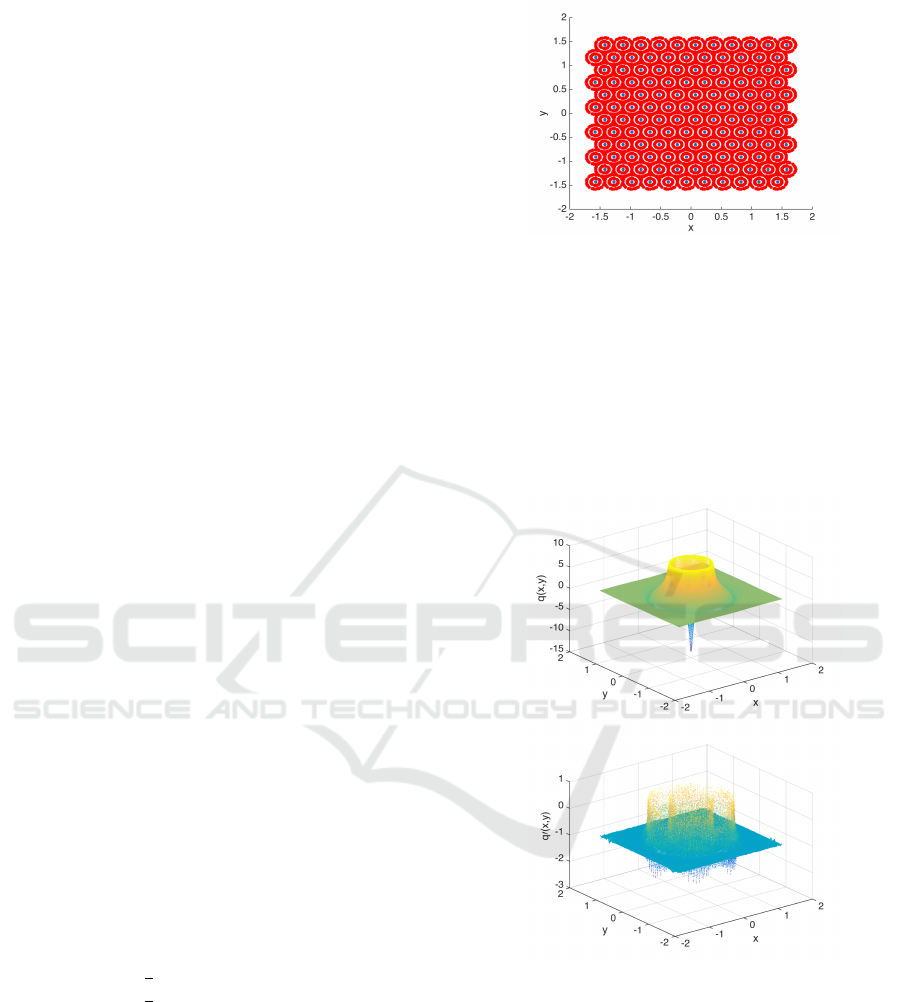
Figure 1: The ﬁgure shows the collocation points (blue)

and the checking points (red) around each collocation point.

The collocations points are used to construct the Lyapunov

function and the checking points are used to evaluate the

orbital derivative of the complete Lyapunov function.

3. Compute the approximate solution v of V

(x) =

−1 for x ∈ X

−

and V

(x) = 0 for x ∈ X

4. Repeat steps 2. and 3. until no more points are

added to X

Figure 2: Lyapunov function for (4). The upper ﬁgure

shows the approximated complete Lyapunov function. The

lower ﬁgure shows its orbital derivative. The minima in the

upper ﬁgure correspond to the asymptotically stable equi-

librium and periodic orbit with radius 1, while the maxi-

mum is attained at the repelling periodic orbit of radius 1/2.

The orbital derivative fails to be negative on the periodic or-

bits and the equilibrium.

Analysing Dynamical Systems - Towards Computing Complete Lyapunov Functions

137

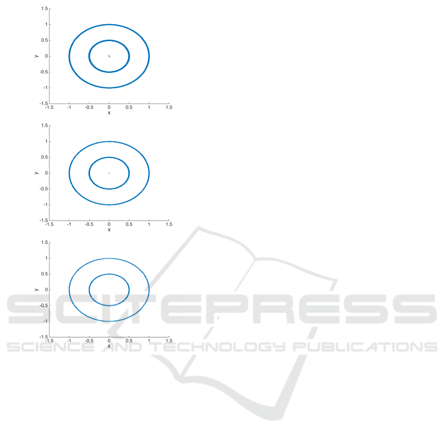
Figure 3: The ﬁgures show the checking points x around

each collocation point, where v

(x) > γ for different values

of γ. Upper: γ = −0.5. Middle: γ = −0.25. Lower: γ = 0.

In all cases, α = 0.02, r = 0.5.

4 EXAMPLES

In the following we apply the method to three exam-

ples and then analyse the behaviour of the method

with respect to certain parameters. In this section we

only consider the ﬁrst step of the method, and we will

discuss the iterations in Section 5. Note that in all

examples we use the notation x = (x,y).

4.1 Two Circular Periodic Orbits

We consider system (1) with right-hand side

f(x,y) =



−x(x

+ y

− 1/4)(x

+ y

− 1) − y

−y(x

+ y

− 1/4)(x

+ y

− 1) + x



(4)

which has an asymptotically stable equilibrium at the

origin, an asymptotically stable periodic orbit with ra-

dius 1, and a repelling periodic orbit with radius 1/2.

To compute the Lyapunov function with our

method we used ψ

5,3

as Wendland function with c =

1. The collocation points were set in (−1.5,1.5) ×

(−1.5,1.5) ⊂ R

and we used α = 0.02.

In Figure 2 we see how the derivative fails to

be negative in both periodic orbits and the equilib-

rium. In the next step of the algorithm, we use points

around each collocation points to check whether the

orbital derivative is above the critical value γ. Figure

3 shows the results for different values of γ, namely

γ = 0,−0.25,−0.5 and a ﬁxed scaling parameter r =

0.5 for (3).

Clearly, γ = 0 is not enough to ﬁnd all failing

points, since some chain-recurrent sets, such as the

equilibrium at the origin, are not detected.

4.2 Van Der Pol Oscillator System

We consider system (1) with right-hand side

f(x,y) =



(1 − x

)y − x



. (5)

System (5) is the two dimensional form of the Van der

Pol oscillator. This describes the behaviour of a non-

conservative oscillator reacting to a non-linear damp-

ing. The origin is an unstable focus, and the system

has an asymptotically stable periodic orbit.

We used our method with the Wendland function

4,2

and c = 1. The collocation points were set in

(−4,4) × (−4,4) ⊂ R

with α = 0.1.

In Figure 4 we see how the derivative fails to be neg-

ative at the points of the periodic orbit. In Figure

5 we show the points in X

for three critical val-

ues γ = 0,−0.25,−0.5 and a ﬁxed scaling parameter

r = 0.5.

For γ = 0 and γ = −0.25 we do not detect all points

of the periodic orbit, but we can already see its shape

(see Figure 5), while for γ = −0.5 the whole periodic

orbit is covered. However, we obtain points in the

gradient-like ﬂow where the orbital derivative fails to

be negative, and thus overestimate the chain-recurrent

set.

4.3 Homoclinic Orbit

We consider system (1) with right-hand side f(x, y) =



x(1 − x

− y

) − y((x − 1)

+ (x

+ y

− 1)

)

y(1 − x

− y

) + x((x − 1)

+ (x

+ y

− 1)

)



(6)

This system has an unstable focus at the origin and

an asymptotically stable homoclinic orbit at a circle

centered at the origin and with radius 1.

SIMULTECH 2017 - 7th International Conference on Simulation and Modeling Methodologies, Technologies and Applications

138

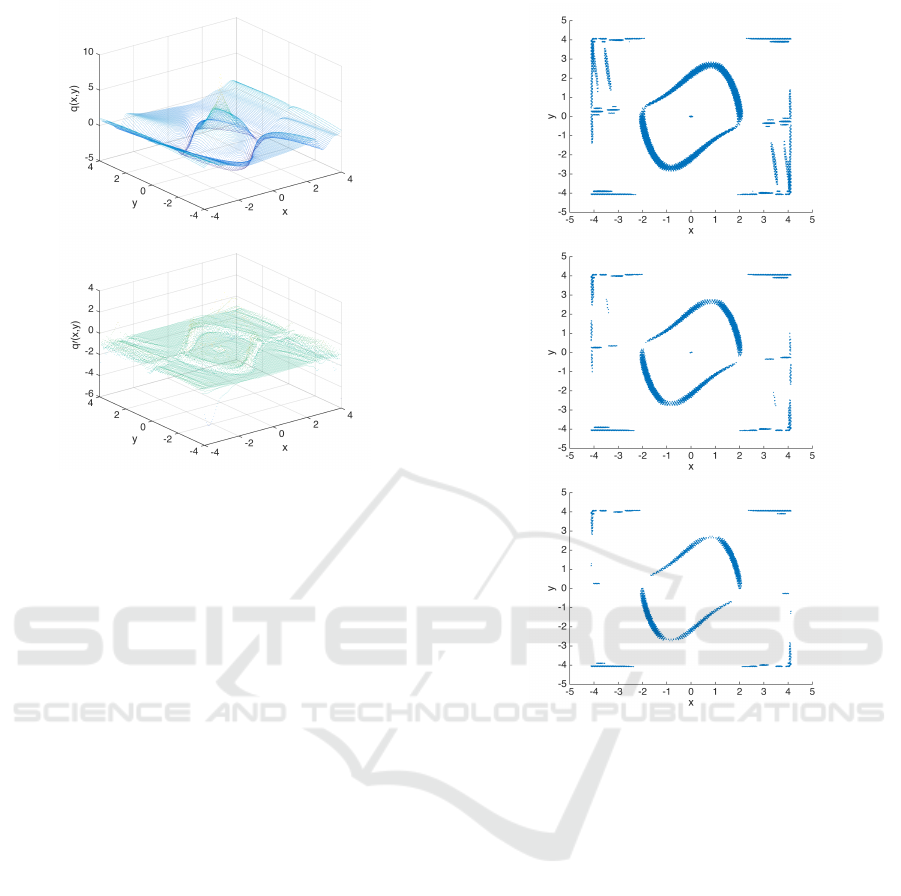
Figure 4: Approximated complete Lyapunov function for

(5). The upper ﬁgure shows the complete Lyapunov func-

tion; the minimum corresponds to the asymptotically stable

periodic orbit and the maximum to the unstable equilibrium

at the origin. The lower ﬁgure shows the orbital derivative

of the complete Lyapunov function. The collocation points

in both cases have α = 0.1. The lower ﬁgure is able to detect

the periodic orbit.

We use our method with the Wendland function

4,2

and c = 1. The collocation points were set in

(−1.5,1.5) × (−1.5,1.5) ⊂ R

with α = 0.02.

The method detects the points of the homoclinic orbit

well, but has problems at the unstable equilibrium at

(1,0), corresponding to the homoclinic orbit. Here,

the approximation also fails at points which belong to

the gradient-like ﬂow.

In Figure 7 we see how the derivative fails to be

negative at the points of the homoclinic orbit, and also

beyond. We show the points in X

for three critical

values γ = 0, −0.25,−0.5 and a ﬁxed scaling radio

r = 0.5.

4.4 Dependence on the Collocation Grid

and the Veriﬁcation Points

A very interesting behaviour is observed by varying

the density of the collocation grid. A natural way to

vary it is by changing the value of the parameter α in

(3): the larger the α the fewer collocation points we

have for a deﬁned area.

In Figure 8 we can observe how our algorithm

converges to the chain-recurrent set for example (4).

We observe that in order to be able to detect the dy-

Figure 5: The ﬁgures show the points x around each collo-

cation point, where v

(x) > γ for different values of γ. Up-

per: γ = −0.5. Middle: γ = −0.25. Lower: γ = 0. In all

cases, α = 0.1, r = 0.5.

namical behaviour, the collocation grid needs to be

sufﬁciently dense. This corresponds to error estimates

between the solution of a PDE and its approximation

using mesh-free collocation which proves that the er-

ror is bounded by a constant times the ﬁll distance,

measuring the density of the collocation points. In

our case, however, the PDE does not have a solution

and thus these error estimates do not apply.

In Figure 9 we consider example (6) and vary the

radius r for the checking points, used to determine

poor and good collocation points. We are only able to

detect the whole homoclinic orbit with a sufﬁciently

large radius. This is to be expected, since at the col-

location points we have v

(x) = −1 and since v

continuous it will be negative close enough to the col-

location points.

Analysing Dynamical Systems - Towards Computing Complete Lyapunov Functions

139

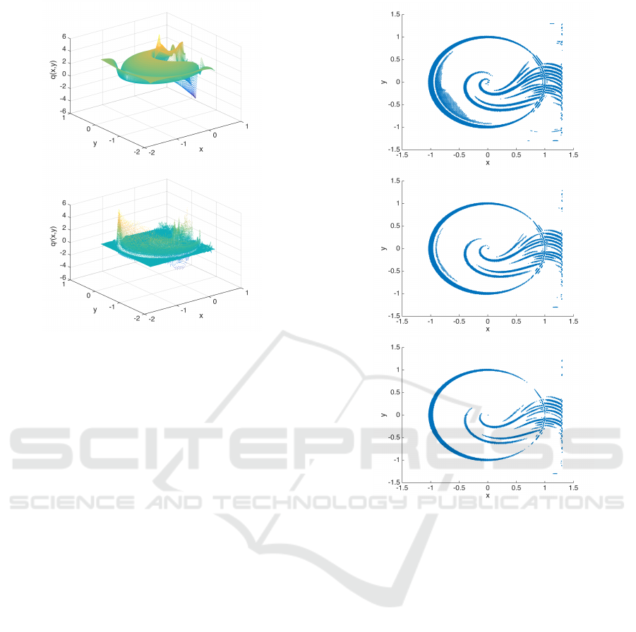
Figure 6: Approximated complete Lyapunov function for

(6). The upper ﬁgure shows the approximated complete

Lyapunov function; the homoclinic orbit corresponds to the

minimum, while the origin is a maximum. The lower ﬁgure

shows its orbital derivative. The collocation points in both

cases have α = 0.02.

5 ITERATION STEPS OF THE

ALGORITHM

After splitting the set of collocation points X into the

set X

, where the approximation is poor, and the re-

maining points X

−

, in the next step, our method will

solve the problem V

(x) = 0 for x ∈ X

and V

(x) =

−1 for x ∈ X

−

. This is done by solving Aβ = r with

an updated right-hand-side r and we look again for

collocation points where the approximation is poor.

This procedure should then be iterated until no more

collocation points are added to X

For the Van der Pol system (5) the results of this

procedure with γ = −0.25 and α = 0.1 can be seen

in Figures 10 to 12. Figure 10 shows the complete

Lyapunov v for each step, which does not change sig-

niﬁcantly after the ﬁrst step; observe, that the range

of v is slightly reduced. Figure 11 shows its orbital

derivative; again, there is no signiﬁcant change after

the ﬁrst step, only the range of v

is slightly reduced

and the values near the chain-recurrent set are now 0

rather than different values above the critical value.

Figure 12, ﬁnally, displays the set of checking

points where the orbital derivative is larger than the

critical value γ = −0.25; these points should approx-

imate the chain-recurrent set, in this case the unstable

equilibrium at the origin and the asymptotically sta-

Figure 7: The ﬁgures show the points x around each collo-

cation point, where v

(x) > γ for different values of γ. Up-

per: γ = −0.5. Middle: γ = −0.25. Lower: γ = 0. In all

cases, α = 0.02, r = 0.5.

ble periodic orbit. We observe that the set of points

increases and nearly covers the whole periodic or-

bit. However, collocation points away from the chain-

recurrent set also are included, mainly at the bound-

ary of the domain under consideration as the values of

(x) become more extreme.

After the ﬁrst step there is no signiﬁcant change

in the ﬁgures, although a close study reveals that the

algorithm still adds points, see Table 1. There are

boundary effects, such that points near the boundary

of the considered domain do not behave as expected.

We are currently studying these phenomena and ex-

pect that a more elaborate way of ﬁxing the values of

at the collocation points will improve the perfor-

mance of the method.

For all examples (4) to (6) we show a table of how

many points we ﬁnd by iterating this procedure. The

corresponding parameters are given in Table 2.

In Table 1 the number of total collocation points and

SIMULTECH 2017 - 7th International Conference on Simulation and Modeling Methodologies, Technologies and Applications

140

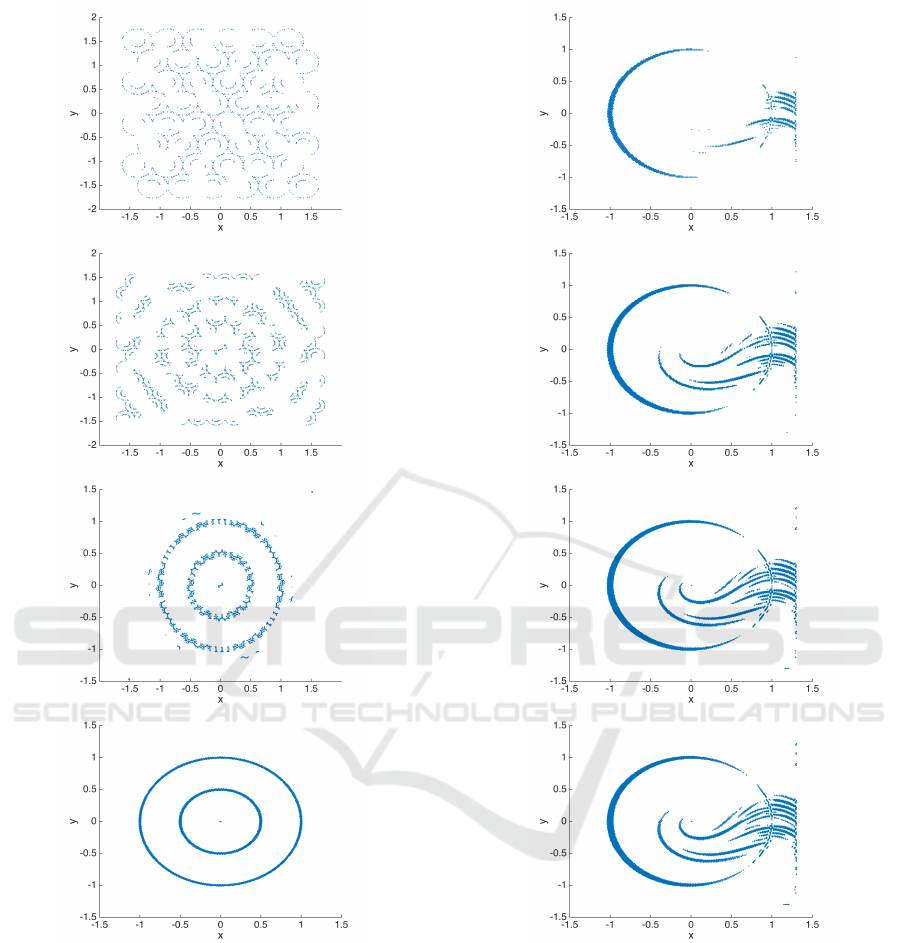
Figure 8: Example (4) with collocation grids of varying

density. Upper α = 0.5. Middle up α = 0.3. Middle down

α = 0.1. Lower α = 0.02. The radii for the test circles for

all of them were set to r = 0.5 and the critical value was

γ = −0.25.

the total number of points in X

with poor approxi-

mation in each step iteration are shown. For system

(4) we see that after the fourth step no more points

are added to X

, while for the other two examples the

method keeps adding points.

Figure 9: We consider example (6) with ﬁxed α = 0.02,

ﬁxed critical value γ = 0.0 and varying r. Upper r = 0.2.

Middle up r = 0.3. Middle down r = 0.4. Lower r = 0.5.

6 CONCLUSIONS AND

OUTLOOK

We have presented a method to compute a complete

Lyapunov function and thus to determine the quali-

tative behaviour of a given ODE, using both the val-

ues of the complete Lyapunov function and its orbital

derivative. A complete Lyapunov function V is con-

stant along solutions in the chain-recurrent set, i.e. the

Analysing Dynamical Systems - Towards Computing Complete Lyapunov Functions

141

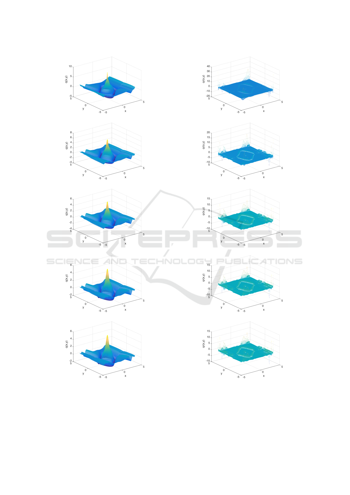
Figure 10: Evolution of the complete Lyapunov function

approximation v(x) for the Van der Pol problem with critical

value γ = −0.25, α = 0.1, r = 0.5. The top ﬁgure shows the

ﬁrst iteration of the method, the second, third and fourth

show the corresponding iterations. The ﬁgures only change

very slightly after the ﬁrst step; one can observe that the

range of values is reduced.

Figure 11: Evolution of the complete Lyapunov function

approximation v

(x) for the Van der Pol problem for the

steps of the method. After the ﬁrst step, where points with

poor approximation have orbital derivatives with positive

values, they are close to zero in subsequent steps. There are

no signiﬁcant changes in the later steps.

SIMULTECH 2017 - 7th International Conference on Simulation and Modeling Methodologies, Technologies and Applications

142

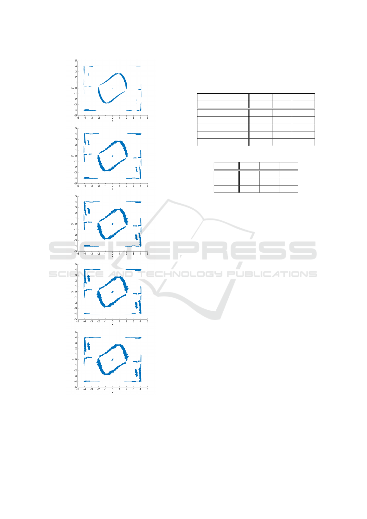
Figure 12: Evolution of the checking points with orbital

derivative larger than the critical value γ = −0.25 for the

Van der Pol problem over several steps. It can be seen

that after the ﬁrst step visibly more points are added, which

nearly cover the whole periodic orbit, while in later steps

there are no signiﬁcant changes. Apart from the chain-

recurrent sets, also points at the boundary of the domain

are marked as poor approximations.

Table 1: In this table we list the overall number of colloca-

tion points as well as the collocation points in X

in each

step of the algorithm for each of the examples (4) to (6). In

example (4), no further points are added after step 4, while

for the other two examples we keep adding points to X

system (4) (5) (6)

collocation points 29440 7708 19500

step 1 1358 762 2517

step 2 1362 956 2751

step 3 1368 1034 2802

step 4 1370 1072 2820

step 5 1370 1092 2829

Table 2: Parameters to obtain results shown in table 1.

system (4) (5) (6)

α 0.02 0.1 0.02

γ -0.25 -0.25 0

r 0.5 0.5 0.5

orbital derivative is zero (V

(x) = 0), and it is strictly

decreasing along solutions in the gradient-like set, i.e.

(x) < 0. Minima of the complete Lyapunov func-

tion correspond to attractors and maxima to repellers.

The method approximately solves the PDE

(x) = −1 with mesh-free collocation. As this PDE

does not have a solution in the chain-recurrent set,

we examine where the approximation is poor (the set

) and thus can determine the chain-recurrent set.

In the subsequent steps of the algorithm we adjust

the PDE problem by solving V

(x) = 0 for x ∈ X

and V

(x) = −1 elsewhere to approximate a complete

Lyapunov function.

While the method works well in several exam-

ples to detect the dynamical behaviour, it does not

always converge to a ﬁxed set of points in X

and

−

= X \ X

, but keeps on adding points. Further-

more, points at the boundary of the domain are in-

cluded in X

, although they belong to the gradient-

like part. The reason could be that we set the or-

bital derivative to 0 and −1, rather than a continuous

function. Further research will consider replacing this

with a more elaborate method, e.g. by replacing the

jump function by a smooth function of the distance to

the detected chain-recurrent set.

ACKNOWLEDGEMENTS

First author in this paper is supported by the Ice-

landic Research Fund (Rann

ıs) grant number 163074-

052, Complete Lyapunov functions: Efﬁcient numer-

ical computation. Special thanks to Dr. Jean-Claude

Berthet for all his good comments and advices on

C++.

Analysing Dynamical Systems - Towards Computing Complete Lyapunov Functions

143

REFERENCES

Anderson, J. and Papachristodoulou, A. (2015). Advances

in computational Lyapunov analysis using sum-of-

squares programming. Discrete Contin. Dyn. Syst. Ser.

B, 20(8):2361–2381.

Auslander, J. (1964). Generalized recurrence in dynamical

systems. Contr. to Diff. Equ., 3:65–74.

Ban, H. and Kalies, W. (2006). A computational approach

to Conley’s decomposition theorem. J. Comput. Non-

linear Dynam, 1(4):312–319.

ornsson, J., Giesl, P., and Hafstein, S. (2014a). Al-

gorithmic veriﬁcation of approximations to complete

Lyapunov functions. In Proceedings of the 21st In-

ternational Symposium on Mathematical Theory of

Networks and Systems, pages 1181–1188 (no. 0180),

Groningen, The Netherlands.

ornsson, J., Giesl, P., Hafstein, S., Kellett, C., and Li,

H. (2014b). Computation of continuous and piece-

wise afﬁne Lyapunov functions by numerical approx-

imations of the Massera construction. In Proceedings

of the CDC, 53rd IEEE Conference on Decision and

Control, Los Angeles (CA), USA.

ornsson, J., Giesl, P., Hafstein, S., Kellett, C., and Li, H.

(2015). Computation of Lyapunov functions for sys-

tems with multiple attractors. Discrete Contin. Dyn.

Syst. Ser. A, 35(9):4019–4039.

Conley, C. (1978a). Isolated Invariant Sets and the Morse

Index. CBMS Regional Conference Series no. 38.

American Mathematical Society.

Conley, C. (1978b). Isolated Invariant Sets and the Morse

Index. CBMS Regional Conference Series no. 38.

American Mathematical Society.

Conley, C. (1988). The gradient structure of a ﬂow i. Er-

godic Theory Dynam. Systems, 8:11–26.

Dellnitz, M., Froyland, G., and Junge, O. (2001). The algo-

rithms behind GAIO – set oriented numerical methods

for dynamical systems. In Ergodic theory, analysis,

and efﬁcient simulation of dynamical systems, pages

145–174, 805–807. Springer, Berlin.

Dellnitz, M. and Junge, O. (2002). Set oriented numer-

ical methods for dynamical systems. In Handbook

of dynamical systems, Vol. 2, pages 221–264. North-

Holland, Amsterdam.

Doban, A. (2016). Stability domains computation and sta-

bilization of nonlinear systems: implications for bio-

logical systems. PhD thesis: Eindhoven University of

Technology.

Doban, A. and Lazar, M. (2016). Computation of Lyapunov

functions for nonlinear differential equations via a

Yoshizawa-type construction. IFAC-PapersOnLine,

49(18):29 – 34. 10th IFAC Symposium on Nonlinear

Control Systems NOLCOS 2016, Monterey, Califor-

nia, USA, 23-25 August 2016.

Giesl, P. (2007). Construction of Global Lyapunov Func-

tions Using Radial Basis Functions. Lecture Notes in

Math. 1904, Springer.

Giesl, P. and Hafstein, S. (2015). Review of computational

methods for Lyapunov functions. Discrete Contin.

Dyn. Syst. Ser. B, 20(8):2291–2331.

Giesl, P. and Wendland, H. (2007). Meshless collocation:

error estimates with application to Dynamical Sys-

tems. SIAM J. Numer. Anal., 45(4):1723–1741.

Goullet, A., Harker, S., Mischaikow, K., Kalies, W., and

Kasti, D. (2015). Efﬁcient computation of Lyapunov

functions for Morse decompositions. Discrete Contin.

Dyn. Syst. Ser. B, 20(8):2419–2451.

Hafstein, S. (2007). An algorithm for constructing Lya-

punov functions. Monograph. Electron. J. Diff. Eqns.

Hsu, C. S. (1987). Cell-to-cell mapping, volume 64 of Ap-

plied Mathematical Sciences. Springer-Verlag, New

York.

Hurley, M. (1992). Noncompact chain recurrence and at-

traction. Proc. Amer. Math. Soc., 115:1139–1148.

Hurley, M. (1995). Chain recurrence, semiﬂows, and gradi-

ents. J Dyn Diff Equat, 7(3):437–456.

Hurley, M. (1998). Lyapunov functions and attractors

in arbitrary metric spaces. Proc. Amer. Math. Soc.,

126:245–256.

Johansen, T. (2000). Computation of Lyapunov functions

for smooth, nonlinear systems using convex optimiza-

tion. Automatica, 36:1617–1626.

Johansson, M. (1999). Piecewise Linear Control Systems.

PhD thesis: Lund University, Sweden.

Kalies, W., Mischaikow, K., and VanderVorst, R. (2005).

An algorithmic approach to chain recurrence. Found.

Comput. Math, 5(4):409–449.

Kamyar, R. and Peet, M. (2015). Polynomial optimization

with applications to stability analysis and control – an

alternative to sum of squares. Discrete Contin. Dyn.

Syst. Ser. B, 20(8):2383–2417.

Krauskopf, B., Osinga, H., Doedel, E. J., Henderson, M.,

Guckenheimer, J., Vladimirsky, A., Dellnitz, M., and

Junge, O. (2005). A survey of methods for computing

(un)stable manifolds of vector ﬁelds. Internat. J. Bifur.

Chaos Appl. Sci. Engrg., 15(3):763–791.

Lyapunov, A. M. (1992). The general problem of the sta-

bility of motion. Internat. J. Control, 55(3):521–790.

Translated by A. T. Fuller from

Edouard Davaux’s

French translation (1907) of the 1892 Russian orig-

inal, With an editorial (historical introduction) by

Fuller, a biography of Lyapunov by V. I. Smirnov, and

the bibliography of Lyapunov’s works collected by J.

F. Barrett, Lyapunov centenary issue.

Marin

osson, S. (2002). Lyapunov function construction for

ordinary differential equations with linear program-

ming. Dynamical Systems: An International Journal,

17:137–150.

Narcowich, F. J., Ward, J. D., and Wendland, H. (2005).

Sobolev bounds on functions with scattered zeros,

with applications to radial basis function surface ﬁt-

ting. Mathematics of Computation, 74:743–763.

Osipenko, G. (2007). Dynamical systems, graphs, and al-

gorithms. Springer, Berlin. Lecture Notes in Mathe-

matics 1889.

Wendland, H. (1998). Error estimates for interpolation by

compactly supported Radial Basis Functions of mini-

mal degree. J. Approx. Theory, 93:258–272.

Wendland, H. (2005). Scattered data approximation, vol-

ume 17 of Cambridge Monographs on Applied and

Computational Mathematics. Cambridge University

Press, Cambridge.

SIMULTECH 2017 - 7th International Conference on Simulation and Modeling Methodologies, Technologies and Applications

144