Wendland Functions
A C++ Code to Compute Them
Carlos Arg
´
aez
1
, Sigurdur Hafstein
1
and Peter Giesl
2
1
Faculty of Physical Sciences, University of Iceland, 107 Reykjav
´
ık, Iceland
2
Department of Mathematics, University of Sussex, Falmer BN1 9QH, U.K.
Keywords:
Radial Basis Functions, Wendland Functions, Compact Support.
Abstract:
In this paper we present a code in C++ to compute Wendland functions for arbitrary smoothness parameters.
Wendland functions are compactly supported Radial Basis Functions that are used for interpolation of data or
solving Partial Differential Equations with mesh-free collocation. For the computations of Lyapunov functions
using Wendland functions their derivatives are also needed so we include this in the code. Wendland functions
with a few fixed smoothness parameters are included in some C++ libraries, but for the general case the only
code freely available was implemented in MAPLE taking advantage of the computer algebra system. The
aim of this contribution is to allow scientists to use Wendland functions in their C++ code without having
to implement them themselves. The computed Wendland functions are polynomials and their coefficients
are computed and stored in a vector, which allows for efficient computation of their values using the Horner
scheme.
1 INTRODUCTION
Mesh-free methods, particularly based upon Radial
Basis Functions, provide a powerful tool for solving
interpolation and generalized interpolation problems
efficiently and in any dimension (Buhmann, 2003;
Fasshauer, 2007; Schaback and Wendland, 2006). An
interpolation problem is, given N pairwise distinct
sites x
1
,...,x
N
∈ R
n
(collocation points) and cor-
responding values f
1
,..., f
N
∈ R to find a function
f : R
n
→ R satisfying f (x
j
) = f
j
for all j = 1,...,N.
For a generalized interpolation problem, instead
of prescribing the values of the function at given sites,
one is given the values of linear functionals applied to
the function. These include linear Partial Differen-
tial Equations with boundary values. Error estimates
between the generalized interpolant and the true solu-
tion are available and depend on the fill distance, mea-
suring how dense the collocation points are. These
methods are particularly suited for high-dimensional
problems and the use of scattered collocation points,
as they do not require the collocation points to lie on a
structured grid. They have been successfully used in
various applications such as geography, engineering,
neural networks, machine learning and image pro-
cessing. Further applications include solving Partial
Differential Equations (Fornberg and Flyer, 2015), the
construction of Lyapunov functions in dynamical sys-
tems (Giesl, 2007), and high-dimensional integration
(Dick et al., 2013).
A (generalized) interpolation problem looks for
a function in a function space, often a Reproducing
Kernel Hilbert Space. The corresponding kernel can
be defined by a Radial Basis Function. Compactly
supported Radial Basis Functions are given by the
family of Wendland functions, which are polynomi-
als on their support. They have two parameters and
are defined recursively.
In this paper we present a numerical code in C++
to explicitly compute the Wendland function with any
given parameters. Another code, written in MAPLE,
has been given previously in (Zhu, 2012; Schaback,
2011). This code takes advantage of MAPLE subrou-
tines like integration, factor and simplify, etc. Fur-
thermore, libMesh (Kirk et al., 2006) and FOAM-FSI
(Blom et al., ) provide C++ libraries that can be used
to evaluate and provide Wendland functions. How-
ever, these just provide few limited cases of Wendland
functions. In our case, we build a C++ code that in-
cludes all necessary operations to compute any Wend-
land function.
In Section 2 we give an overview over generalized
interpolation and Wendland functions. In Section 3
we describe the algorithm used in the code, and in
Argáez, C., Hafstein, S. and Giesl, P.
Wendland Functions - A C++ Code to Compute Them.
DOI: 10.5220/0006441303230330
In Proceedings of the 7th International Conference on Simulation and Modeling Methodologies, Technologies and Applications (SIMULTECH 2017), pages 323-330
ISBN: 978-989-758-265-3
Copyright © 2017 by SCITEPRESS – Science and Technology Publications, Lda. All rights reserved
323

Section 4 we give some examples of computed Wend-
land functions with our code. The full C++ code is
presented in the appendix.
2 GENERALIZED
INTERPOLATION AND
WENDLAND FUNCTIONS
To discuss generalized interpolation in more detail,
we let H ⊂ C(R
n
,R) be a Hilbert space of functions
f : R
n
→ R, which are at least continuous. Its dual H
∗
consists of all functionals λ : H → R, which are linear
and continuous. Examples of such functionals include
Dirac’s delta distribution δ
x
0
( f ) = f (x
0
), evaluating
the function at the point x
0
∈ R
n
and differential op-
erators evaluated at a point, e.g., λ = δ
x
0
◦
∂
∂x
j
.
The generalized interpolation problem is: given N
linearly independent functionals λ
1
,...,λ
N
∈ H
∗
and
corresponding values f
1
,..., f
N
∈ R, a generalized in-
terpolant is a sufficiently smooth function f : R
n
→ R
satisfying λ
j
( f ) = f
j
for all j = 1, . . . , N. Note that
the usual interpolation problem is a special case with
λ
j
= δ
x
j
.
The norm-minimal interpolant is the interpolant
that, in addition, minimizes the norm of the Hilbert
space, namely min{k f k
H
: λ
j
( f ) = f
j
,1 ≤ j ≤ N}.
It is well-known (Wendland, 2005) that the norm-
minimal interpolant can be represented as a linear
combination of the Riesz representers v
j
∈ H of the
functionals. If the Hilbert space is a Reproducing Ker-
nel Hilbert Space, then these Riesz representers can
be expressed in a simpler way.
A Reproducing Kernel Hilbert Space is a Hilbert
space H with a reproducing kernel Φ : R
n
× R
n
→ R
such that
1. Φ(·,x) ∈ H for all x ∈ R
n
2. g(x) = hg,Φ(·,x)i
H
for all g ∈ H and x ∈ R
n
where h·,·,i denotes the inner product of the Hilbert
space H.
Then the Riesz representers are given v
j
=
λ
y
j
Φ(·,y), i.e. the functional applied to one of the
arguments of the reproducing kernel. Hence, the
norm-minimal interpolant can be written as f (x) =
∑
N
j=1
β
j
λ
y
j
Φ(x,y), where the coefficients β
j
are de-
termined by the interpolation conditions λ
j
( f ) = f
j
,
1 ≤ j ≤ N.
Often kernels depend on the difference between
the two arguments, i.e. Φ(x,y) := φ(x − y). Ra-
dial Basis Functions are radial functions φ, namely
φ(x − y) := Ψ(kx − yk). There are a variety of Ra-
dial Basis Functions, including the Gaussians, multi-
quadrics, inverse multiquadrics and thin plate splines.
Each of them defines a different Reproducing Kernel
Hilbert Space.
Compactly supported Radial Basis Functions,
which are polynomials on their support, were con-
sidered in (Wu, 1995; Schaback and Wu, 1996), and
are now called Wendland functions (Wendland, 1995;
Wendland, 1998); for a discussion of compactly sup-
ported Radial Basis Functions see (Zhu, 2012). The
corresponding Reproducing Kernel Hilbert Space is
norm-equivalent to a Sobolev space.
In this paper, we describe a new algorithm to de-
fine compute Wendland Function of any order.
The Wendland functions ψ
l,k
, where l ∈ N and k ∈
N
0
are defined recursively by (Wendland, 1995)
ψ
l,0
(r) = (1 − r)
l
+
ψ
l,k+1
(r) =
Z
1
r
tψ
l,k
(t)dt for k = 0,1,...
where x
+
=
(
x for x > 0
0 for x ≤ 0
.
So, if we want to evaluate a Wendland function
for given k and l at the point cr, where c > 0 is a fixed
constant, we obtain:
ψ
l,k
(cr) =
Z
1
cr
t
k
Z
1
t
k
t
k−1
...
Z
1
t
2
| {z }
k times
t
1
ψ
l,0
(t
1
)
k times
z }| {
dt
1
...dt
k
(1)
3 ALGORITHM
3.1 Function wendlandfunction
The Wendland function is built up from recursive in-
tegrations of a polynomial. As seen in (1), the param-
eters that define the polynomial’s degree are k and l,
where l denotes the degree of the initial polynomial
and k is the number of recursive integrations. We will
write the algorithm as a C++ program and will use the
libraries Blitz++ and Boost.
In our calculations, we will focus on the calcula-
tion of the polynomial on the support; note that the
support of ψ
l,k
(r) is [0,1]. Furthermore, it is seen in
(1), that in each step we multiply the previous poly-
nomial by a factor t. This product will increase the
degree of the polynomial by one and the integration
will also increase the polynomial’s degree by one.
Hence, the final degree of the Wendland function will
be l + 1 + 2 · k.
Below we will present the steps to construct the
Wendland function.
SIMULTECH 2017 - 7th International Conference on Simulation and Modeling Methodologies, Technologies and Applications
324

1. First, we compute the coefficients of the binomial
expansion of (1−r)
l
using Pascal’s Triangle. The
coefficients are stored in an array (a vector) whose
indexing corresponds to the degree of the respec-
tive polynomial term. In more detail, at the n-th
position we store the coefficient of the term r
n
for
n = 0,. . . , l. The dimension of the storage in this
part of the code will be l + 1.
2. Once the binomial expansion is computed, the
first multiplication t(1 − t)
l
must be performed.
This multiplication will only increase each term’s
degree by one, without affecting the coefficients,
hence, we move the coefficients from the previous
iteration into the next position in the array. So,
the coefficient of t
n
will become the coefficient of
t
n+1
for n = 0,...,l.
3. The integration will also increase the length of the
array by one. The difference is that in this case
the coefficients will be integrated using the simple
formula (without the integration constant):
Z
at
n
dt =
at
n+1
n + 1
Therefore, the coefficient of t
n
will be divided by
n + 1 and stored in the position n + 1 of the new
array.
4. The limits of the integration are r and 1. Evaluat-
ing a polynomial at 1 is achieved by adding up all
coefficients. The lower limit, r will preserve the
terms of the polynomial, but we need to change
the sign. Altogether, the new polynomial will be
N(r)
|{z}
new polynomial
= P(1)
|{z}
polynomial evaluated at 1
− P(r)
|{z}
original polynomial
5. After that, repeat steps 2. to 4. until the last inte-
gration is completed.
6. Finally, we want to evaluate the function ψ
l,k
(cr)
with fixed positive constant c > 0. Hence, at the
last integration, we consider the evaluation of cr
at the lower limit only.
In practice, when the Wendland functions are
computed, they tend to be presented with integer coef-
ficients, i.e. the integration coefficients must be scaled
by their Least Common Multiplayer (LCM). The co-
efficients in C++ are given as double and to be able
to obtain the LCM one needs integers. Furthermore,
the library to compute the LCM is a Boost library that
requires to clearly define the type of the variable. So,
the integrate coefficient are stored as a different ar-
ray defined as long long unsigned. Once the LCM
is obtained, the Greatest Common Divisor (GCD) is
also computed to make sure that the factor to make
the coefficients integers is the least.
The code that computes the Wendland functions
is divided in three parts and can be found in the ap-
pendix.
1. The first step computes the coefficients of Pascal’s
Triangle for the degree l. If k = 0, then the Wend-
land function will be given by (1 − cr)
l
for any
given value of c. If k 6= 0 then the c parameter
will be not considered in this iteration.
2. The next step is to keep track of iterations up
to k − 1, in this section of the code the product
and the integration will be carried out. The vec-
tor momentaneo, i.e.,“momentanous” is created to
store the numerators momentanously.
The term that corresponds to the evaluation of the
upper limit 1, equals the sum of all the terms.
Since in a hand-made calculation, it would be nec-
essary to keep track of the denominators as well,
following that logic, the denominator is equal to
the LCM, i.e. the divisors(0)=mcm of all the el-
ements of divisors.
3. The last iteration is the most difficult one. It is
given when the value of the last iteration k occurs
and k 6= 0. It follows the same logic: the first vec-
tor is the product that equals the coefficients of the
last integration but is stored in the previous entry
plus one. Now the integration is considered with
the c parameter, namely integral(i+1)=
pow(c,i+1)*product(i)/(i+1);.
In the next step, the divisors are computed, then
the LCM and finally divisors(0)=mcm; in this
case, the upper limit 1 will be as before, but now
we are required to divide by the corresponding c
n
:
integral(0)-=integral(i)/pow(c,i);
Yet again the corresponding numera-
tor will be numerators(N+2*k-l-2-j)
=round(integral(0)*divisors(0)); where
the function round ensures that the number is
integer. In order to compute the GCD it is
necessary to figure out that all the numerators
are correct. However, if one is not interested in
making the coefficient integers, the C++ function
here presented is able to give the corresponding
Wendland functions for double coefficients. The
option is a boolean variable, if equals true then the
Wendland function is scaled. Notice that when
k = 0 the c parameter is computed automatically
according to their value.
Furthermore, when one is interested in using a
non-integer c, one can just activate this options
with a second boolean variable that considers c as
integers only when it is true. This is because when
scaling the polynomial coefficients, one should be
carefully to scale them at the proper time.
Wendland Functions - A C++ Code to Compute Them
325

3.2 AUXILIARY FUNCTIONS ψ
1
, ψ
2
Wendland functions find important applications in
algorithms to compute Lyapunov functions (Giesl,
2007). In those, the computation of the derivatives of
Wendland functions is mandatory. For a given Wend-
land function ψ
l,k
(r) =: ψ(r) we define the auxiliary
functions ψ
1
and ψ
2
as follows for r > 0:
ψ
1
(r) =
d
dr
ψ(r)
r
ψ
2
(r) =
d
dr
ψ
1
(r)
r
(2)
Therefore to be able to implement (2), one must
notice that for a given Wendland function the func-
tion ψ
1
will be a polynomial of two degrees lower
than the original Wendland function. For ψ
2
(r) one
should follow the same logic. For r > 0, ψ
2
(r) will
be two orders lower than ψ
1
(r). When evaluating
it, before calling the functions wendlandpsi1 and
wendlandpsi2 one could test r to find whether it is
r > 0 or r = 0. The full C++ codes are presented in
the appendix.
3.3 GENERAL DISCUSSION
This code produces high order Wendland functions
that are stored in a very efficient way by terms of an
array. Such storage allows us to use Wendland func-
tions as many times as required without re-computing.
Furthermore, this allows to evaluate Wendland func-
tion in very efficient ways, e.g., by means of Horner’s
method to evaluate polynomials. In general, the com-
putation of a high order Wendland function with this
code takes a tenth of a millisecond. There are some
advantages and disadvantages that need to be dis-
cussed. On the one hand, the limit of performance of
our code will depend on the capability of any partic-
ular computer to storage long long unsigned vari-
ables. Therefore, although this codes is designed to
provide any Wendland function, it has the disadvan-
tage of reaching only the limit of the local computer
where it is run. On the other hand, it is preferable to
have a code that computes Wendland functions rather
than a library that would, in general, be very limited
in capabilities. To the best of our knowledge current
libraries only provide a limited selection of Wendland
functions.
4 EXAMPLES
All the results here presented, have been tested and
compared with Mathematica.
For c = 1
ψ
3,9
(r) = 2431 − 30030r
2
+ 171171r
4
− 596904r
6
+1424430r
8
− 2469012r
10
+ 3233230r
12
−3325608r
14
+ 2909907r
16
− 3233230r
18
+2752512r
19
− 969969r
20
+ 131072r
21
ψ
4,9
(r) = 221 − 3003r
2
+ 19019r
4
− 74613r
6
+203490r
8
− 411502r
10
+ 646646r
12
−831402r
14
+ 969969r
16
− 1616615r
18
+1835008r
19
− 969969r
20
+ 262144r
21
−29393r
22
ψ
5,9
(r) = 221 − 3289r
2
+ 23023r
4
−100947r
6
+ 312018r
8
− 728042r
10
+1352078r
12
− 2124694r
14
+ 3187041r
16
−7436429r
18
+ 10551296r
19
−7436429r
20
+ 3014656r
21
−676039r
22
+ 65536r
23
ψ
6,9
(r) = 1105 − 17940r
2
+ 138138r
4
−672980r
6
+ 2340135r
8
− 6240360r
10
[phone]r
12
− 25496328r
14
[phone]r
16
− 148728580r
18
[phone]r
19
− 223092870r
20
[phone]r
21
− 40562340r
22
+7864320r
23
− 676039r
24
ψ
7,6
(r) = 11 − 171r
2
+ 1292r
4
−6460r
6
+ 25194r
8
− 92378r
10
+554268r
12
− 1323008r
13
+1662804r
14
− 1323008r
15
+692835r
16
− 233472r
17
+46189r
18
− 4096r
19
ψ
7,9
(r) = 221 − 3900r
2
+ 32890r
4
−177100r
6
+ 688275r
8
− 2080120r
10
+5200300r
12
− 11589240r
14
[phone]r
16
− 106234700r
18
[phone]r
19
− 223092870r
20
[phone]r
21
− 67603900r
22
[phone]r
23
− 3380195r
24
+262144r
25
ψ
8,9
(r) = 17 − 325r
2
+ 2990r
4
−17710r
6
+ 76475r
8
− 260015r
10
+742900r
12
− 1931540r
14
+5311735r
16
− 26558675r
18
[phone]r
19
− 74364290r
20
[phone]r
21
− 33801950r
22
[phone]r
23
− 3380195r
24
+524288r
25
− 37145r
26
For c = 2
ψ
5,4
(r) = 7 − 312r
2
+ 6864r
4
− 109824r
6
+2306304r
8
− 9371648r
9
+ 18450432r
10
−20447232r
11
+ 12300288r
12
− 3145728r
13
SIMULTECH 2017 - 7th International Conference on Simulation and Modeling Methodologies, Technologies and Applications
326

For c = 3
ψ
5,4
(r) = 7 − 702r
2
+ 34749r
4
−1250964r
6
+ 59108049r
8
− 360277632r
9
[phone]r
10
− 1768635648r
11
[phone]r
12
− 612220032r
13
For c = 4
ψ
5,4
(r) = 7 − 1248r
2
+ 109824r
4
−7028736r
6
+ 590413824r
8
−4798283776r
9
+ 18893242368r
10
−41875931136r
11
+ 50381979648r
12
−25769803776r
13
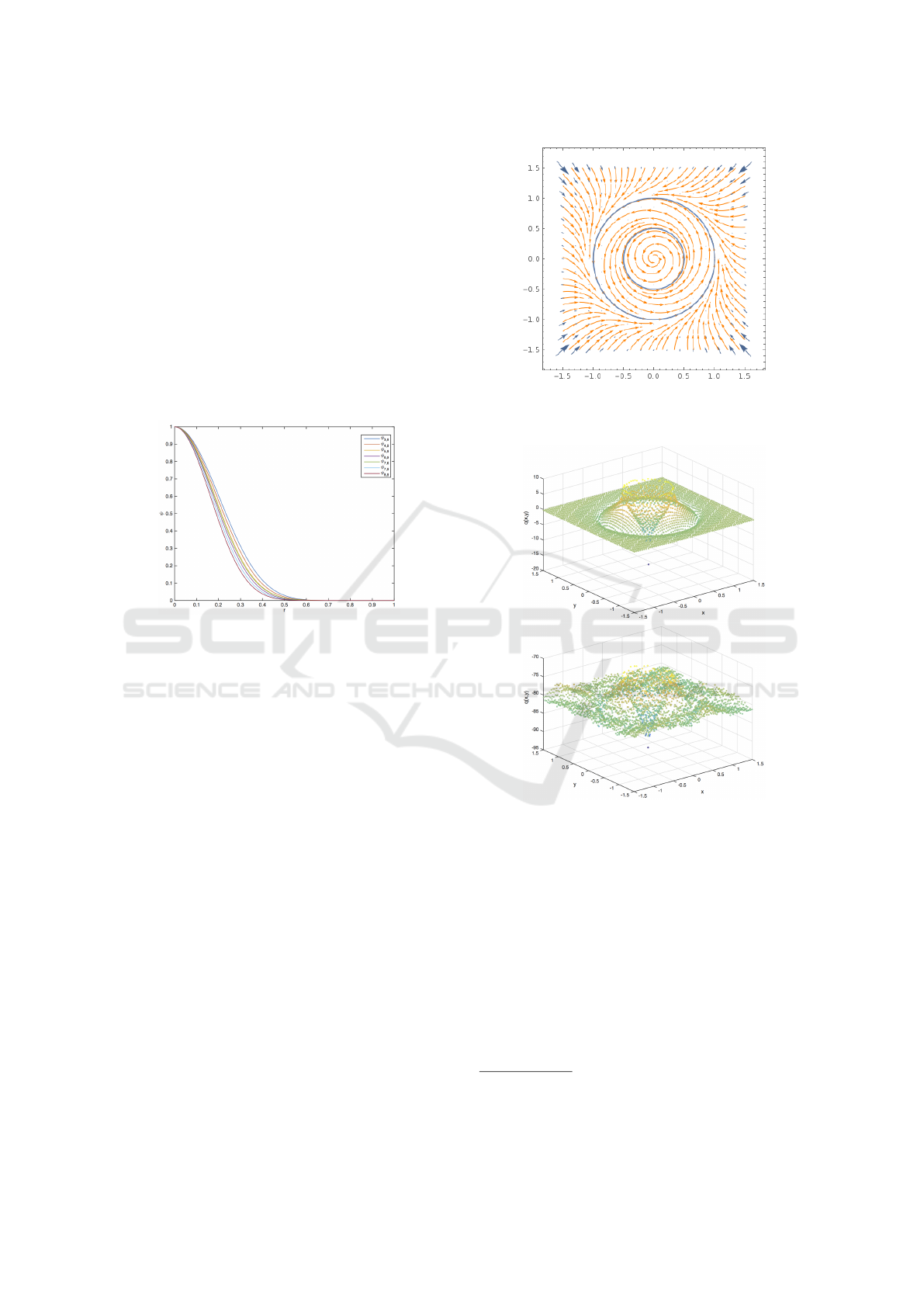
Next, we show how the graphs of these equations look
for c = 1.
Figure 1: Different Wendland functions obtained with this
code. All of them have been normalised and they are pre-
sented over all their support [0,1].
5 APPLICATIONS
Wendland functions have important applications to
compute Lyapunov functions (Giesl, 2007). In the
following, we give examples of computing Lyapunov
functions for a particular system with low and high
order Wendland functions, ψ
5,3
and ψ
9,7
respectively.
We consider the dynamical system given by

˙x
˙y

=

−x(x
2
+ y
2
− 1/4)(x
2
+ y
2
− 1) − y
−y(x
2
+ y
2
− 1/4)(x
2
+ y
2
− 1) + x.

, (3)
System (3) has a repelling periodic orbit with radius
1/2, an asymptotically stable periodic orbit with ra-
dius 1 and the origin is a stable equilibrium.
Obtaining a vector plot of system (3) with Math-
ematica (Wolfram Research, Inc., ), it is possible to
notice how the system behaves, Figure 2.
Now, the computed Lyapunov functions are
shown in Figure 3, while the contour lines for system
(3) are presented in Figure 4.
Figure 2: Vector plot for system (3). The blue line show
both the asymptotically stable periodic orbit with radius 1
and the repelling periodic orbit with radius 1/2.
Figure 3: Approximated Lyapunov functions for system
(3). The upper figure shows the Lyapunov function using
ψ
5,3
(r) and the lower one shows it for ψ
9,7
(r).
6 CONCLUSIONS
In this paper we have presented an efficient im-
plementation to compute the Wendland function
1
ψ
l,k
(cr) for any given parameters l ∈ N, k ∈ N
0
and
c > 0. Wendland functions are compactly supported
Radial Basis Functions that are used to solve (gen-
eralized) interpolation problems in high dimensions.
These include solving PDE boundary value problems
which are used in many important applications.
1
The code can be downloaded directly from:
https://notendur.hi.is/∼carlos/codes/WendlandFunction-
CarlosArgaez2017.zip.
Wendland Functions - A C++ Code to Compute Them
327

Figure 4: Contour lines for the approximated Lyapunov
functions for system (3). The upper figure shows the con-
tour lines for the Lyapunov function using ψ
5,3
(r) and the
lower one shows them for ψ
9,7
(r).
ACKNOWLEDGEMENTS
First author in this paper is supported by the Ice-
landic Research Fund (Rann
´
ıs) grant number 163074-
052, Complete Lyapunov functions: Efficient numer-
ical computation. Special thanks to Dr. Jean-Claude
Berthet for all his good comments and advices on
C++.
REFERENCES
Blom, D., Cardiff, P., Gillebaart, T., t. Hofstede, E., and
Kazemi-Kamyab, V. Foam-fsi project.
Buhmann, M. D. (2003). Radial basis functions: theory
and implementations, volume 12 of Cambridge Mono-
graphs on Applied and Computational Mathematics.
Cambridge University Press, Cambridge.
Dick, J., Kuo, F. Y., and Sloan, I. H. (2013). High-
dimensional integration: the quasi-Monte Carlo way.
Acta Numer., 22:133–288.
Fasshauer, G. E. (2007). Meshfree approximation methods
with MATLAB, volume 6 of Interdisciplinary Mathe-
matical Sciences. World Scientific Publishing Co. Pte.
Ltd., Hackensack, NJ. With 1 CD-ROM (Windows,
Macintosh and UNIX).
Fornberg, B. and Flyer, N. (2015). Solving PDEs with radial
basis functions. Acta Numer., 24:215–258.
Giesl, P. (2007). Construction of Global Lyapunov Func-
tions Using Radial Basis Functions. Lecture Notes in
Math. 1904, Springer.
Kirk, B. S., Peterson, J. W., Stogner, R. H., and Carey, G. F.
(2006). libMesh: A c++ library for parallel adaptive
mesh refinement/coarsening simulations. Engineering
with Computers, 22(3–4):237..254.
Schaback, R. (2011). The missing wendland functions.
34:67–81.
Schaback, R. and Wendland, H. (2006). Kernel techniques:
from machine learning to meshless methods. Acta Nu-
mer., 15:543–639.
Schaback, R. and Wu, Z. (1996). Operators on radial func-
tions. J. Comput. Appl. Math., 73(1-2):257–270.
Wendland, H. (1995). Piecewise polynomial, positive defi-
nite and compactly supported radial functions of min-
imal degree. Adv. Comput. Math., 4(4):389–396.
Wendland, H. (1998). Error estimates for interpolation by
compactly supported Radial Basis Functions of mini-
mal degree. J. Approx. Theory, 93:258–272.
Wendland, H. (2005). Scattered data approximation, vol-
ume 17 of Cambridge Monographs on Applied and
Computational Mathematics. Cambridge University
Press, Cambridge.
Wolfram Research, Inc. Mathematica, wolframalpha.
Wu, Z. M. (1995). Compactly supported positive definite
radial functions. Adv. Comput. Math., 4(3):283–292.
Zhu, S.-X. (2012). Compactly supported radial basis func-
tions: how and why? OCCAM Preprint Number
12/57, University of Oxford, Eprints Archive.
APPENDIX: THE CODE
The complete Wendland Function code is given be-
low:
void wendlandfunction(double l,double k,
double c,bool b, bool d, Array<double, 1>&wdlf)
{
long long unsigned comparing;
long long unsigned mcm = 0;
long long unsigned mcd = 0;
long long unsigned N=l+1;
Array <double, 1> coeff((int)(N+2*k+1)),
cpower((int)(N+2*k+1)),
pascalcoeff((int)(N+2*k+1));
Array <double, 1> integral((int)(N+2*k+1)),
integralbackup((int)(N+2*k+1)),
momentaneo((int)(N+2*k+1));
Array < long long unsigned, 1>
divisors((int)(N+2*k+1)),
numerators(N+2*k);
Array <double, 1> product((int)(N+2*k));
wdlf.resize((int)(N+2*k+1));
numerators=1;
for(int j=0;j<=k;j++)
{
product.reference(Range(0,(int)(N+2*j-2)));
integral.reference(Range(0,(int)(N+2*j-1)));
SIMULTECH 2017 - 7th International Conference on Simulation and Modeling Methodologies, Technologies and Applications
328

integralbackup.reference
(Range(0,(int)(N+2*j-1)));
divisors.reference(Range(0,(int)(N+2*j-1)));
divisors=1.0;
product=0.0;
integral=0.0;
cpower=0.0;
if(j==0)
{
if(k>0.0)
{
wdlf.reference(Range(0,l));
for(int i=0;i<=l;i++)
{
integral.reference(Range(0,l));
integralbackup.reference(Range(0,l));
cpower(i)=i;
double x=1;
for(int h=0;h<=i;h++)
{
coeff(h)=pow(-1,h)*x;
x = x * (i - h) / (h + 1);
}
}
integral=coeff;
for(int i=0; i<l+1; i++)
{
numerators(numerators.size()-l+i-1)
=coeff(i);
}
}else{
for(int i=0;i<=l;i++)
{
integral.reference(Range(0,l));
integralbackup.reference(Range(0,l));
cpower(i)=i;
double x=1;
for(int h=0;h<=i;h++)
{
coeff(h)=pow(c,cpower(h))*pow(-1,h)*x;
x = x * (i - h) / (h + 1);
}
}
integral=coeff;
}
momentaneo=1.0;
}if((j>0) && (j<k)){
for(int i=0; i<product.size()-1; i++)
{
product(i+1)=coeff(i);
}
for(int i=1; i<integral.size()-1; i++)
{
integral(i+1)=product(i)/(i+1);
}
for(int i=(int)integral.size()-1; i>=2; i--)
{
divisors(i)=(i)*momentaneo(i-2);
}
mcm=divisors(0);
for(int i=0; i<=divisors.size()-1; i++)
{
mcm
=boost::math::lcm(mcm,divisors(i));
}
divisors(0)=mcm;
for(int i=1; i<integral.size(); i++)
{
integral(0)-=integral(i);
}
integral=-1.0*integral;
numerators(N+2*k-l-2-j)
=round(integral(0)*divisors(0));
coeff.reference
(Range(0,(int)integral.size()-1));
wdlf.reference
(Range(0,(int)integral.size()-1));
momentaneo.reference
(Range(0,(int)integral.size()-1));
momentaneo=divisors;
coeff=integral;
}if((j==k) && (k!=0)){
for(int i=0; i<product.size()-1; i++)
{
product(i+1)=coeff(i);
}
for(int i=1; i<integral.size()-1; i++)
{
integral(i+1)=pow(c,i+1)*product(i)/(i+1);
}
for(int i=(int)integral.size()-1; i>=2; i--)
{
divisors(i)=(i)*momentaneo(i-2);
}
mcm=divisors(0);
for(int i=0; i<=(int)divisors.size()-1; i++)
{
mcm=
boost::math::lcm(mcm,divisors(i));
}
divisors(0)=mcm;
for(int i=1; i<integral.size(); i++)
{
integral(0)-=integral(i)/pow(c,i);
}
integral=-1.0*integral;
numerators(N+2*k-l-2-j)
=round(integral(0)*divisors(0));
if(numerators(N+2*k-l-2-j)==0)
{
numerators(N+2*k-l-2-j)=1;
}
for(int i=0; i<integral.size()-1;i++)
{
if(integral(i)==0.0)
{
numerators(i)=integral(i);
}
}
mcm=divisors(0);
for(int i=1; i<=divisors.size()-1; i++)
{
mcm=
boost::math::lcm(mcm,divisors(i));
Wendland Functions - A C++ Code to Compute Them
329

}
divisors(0)=mcm;
numerators(0)=round(divisors(0)*integral(0));
for(int i=0; i<=divisors.size()-1; i++)
{
mcd=
boost::math::gcd(numerators(i),divisors(i));
divisors(i)=divisors(i)/mcd;
}
mcm=divisors(0);
for(int i=1; i<=divisors.size()-1; i++)
{
mcm=
boost::math::lcm(mcm,divisors(i));
}
coeff.reference
(Range(0,(int)integral.size()-1));
wdlf.reference
(Range(0,(int)integral.size()-1));
momentaneo.reference
(Range(0,(int)integral.size()-1));
momentaneo=divisors;
coeff=integral;
}
}
if(k==0)
{
if(b)
{
wdlf=integral;
}else{
wdlf=integral;
}
}else{
integralbackup=integral;
if(b)
{
cout << "mcm " << mcm << endl;
for(int i=0; i<(int)integral.size();i++)
{
cout.precision(18);
wdlf(i)=round(mcm*integral(i));
}
Array<double, 1> wdlfm((int)integral.size());
wdlfm=wdlf;
long long unsigned mcd=wdlfm(0);
for(int i=1; i<(int)integral.size();i++)
{
if(wdlf(i)!=0.0)
{
comparing=abs(wdlf(i));
mcd=
boost::math::gcd(mcd,comparing);
}
}
cout << "mcd " << mcd << endl;
if(d)
{
for(int i=0; i<(int)integral.size();i++)
{
wdlf(i)=(wdlfm(i)/mcd);
}
}else{
for(int i=0; i<(int)integral.size();i++)
{
wdlf(i)=mcm*(integralbackup(i)/mcd);
}
}
}else{ wdlf=integral; }
}
The code for the auxiliary function ψ
1
:
void wendlandpsi1(Array<double, 1>
&wdlfinput, Array<double, 1> &wdlf1)
{
int dim=(int)wdlfinput.size();
wdlf1.resize(dim-2);
for(int i=dim-1; i>0; i--)
{ wdlf1(i-2)=i*wdlfinput(i); }
}
The code for the auxiliary function ψ
2
:
void wendlandpsi2(Array<double, 1>
&wdlf1, Array<double, 1> &wdlf2)
{
int dim=(int)wdlf1.size();
wdlf2.resize(dim-2);
for(int i=dim-1; i>0; i--)
{ wdlf2(i-2)=i*wdlf1(i); }
}
SIMULTECH 2017 - 7th International Conference on Simulation and Modeling Methodologies, Technologies and Applications
330