
Arbitrary Trajectory Foot Planner for Bipedal Walking
Ramil Khusainov
1
, Artur Sagitov
2
, Alexandr Klimchik
1
and Evgeni Magid
2
1
Intelligent Robotic Systems Laboratory, Innopolis University, Innopolis City, Russian Federation
2
Higher Institute of Information Technology & Information Systems, Kazan Federal University, Kazan,
Russian Federation
Keywords: Foot Planner, Zero Moment Point, Preview Control.
Abstract: This paper presents a foot planner algorithm for bipedal walking along an arbitrary curve. It takes a
parametrically defined desired path as an input and calculates feet positions and orientations at each step.
Number of steps that are required to complete the path depends on a maximum step length and maximum foot
rotation angle at each step. Provided with results of the foot planner, our walking engine successfully performs
robot locomotion. Verification tests were executed with AR601M humanoid robot.
1 INTRODUCTION
Nowadays the interest to humanoid robots rapidly
increases. A significant number of successful
humanoid solutions and experiments have been
demonstrated in the past decades by different research
groups and companies, including such as ASIMO
(Sakagami et al., 2002), ATLAS (Feng et al., 2015),
HRP-4C (Kajita et al., 2010), Wabian (Ogura et al.,
2006), AR601M (Khusainov et al., 2015) and others
(Shamsuddin et al., 2011) (Ha et al., 2011). However,
bipedal robot walking still remains a challenging
research topic due to its complexity. One of the most
ambitious goals is creating a universal robot that
could operate in dynamic environments and replace a
human in dangerous operations, e.g., supporting
astronauts during space flights or acting in a
proximity of a nuclear energy source, chemically or
biologically contaminated environments. An obvious
advantage of anthropomorphic robots is their ability
to apply humanlike skills in order to utilize existing
human-oriented technologies and devices. Thus,
robust omnidirectional locomotion of a bipedal robot
in environments with obstacles becomes crucial to
perform such operations effectively.
Robot autonomous performance is another
important issue since human teleoperation is not
always possible. In order to increase robot
capabilities different simultaneous localization and
mapping (SLAM) algorithms are used (Stasse et al.,
2006). Robot stereo cameras or laser scanners are
used to detect surrounding objects and find robot
relative position. Such algorithms can generate an
optimal and safe trajectory from an initial location to
a goal location (Figure1). Next, the robot should
generate steps’ pattern along the given trajectory
based on robot kinematic constraints so that a walking
engine could utilize this pattern to perform stable
locomotion.
For example in (Strom et al., 2010) authors
demonstrated an omnidirectional walking foot
planner for NAO robot. In (Zhao et al., 2012) 3D foot
planner was demonstrated, which enables robot to
maneuver through 3D structures. In (Chestnutt et al.,
2005) authors present a footstep planner for the
Honda ASIMO robot. However, the effect of
kinematic limits in robot leg joints on step parameters
has not been studied thoroughly.
In our work we developed an algorithm that
generates desired foot positions of the robot for any
given trajectory of motion taking into account
kinematic limits in robot legs. Then a foot pattern is
fed to preview control approach based walking
engine, which provides walking along arbitrary
trajectory. Additionally, we estimate errors in
position and orientation upon reaching the goal
location.
The rest of the paper is organized as following.
Section 2 describes a foot planner algorithm. Section
3 presents a biped robot walking engine. Section 4
demonstrates experiment results. Finally, Section 5
presents conclusions and future work.
Khusainov, R., Sagitov, A., Klimchik, A. and Magid, E.
Arbitrary Trajectory Foot Planner for Bipedal Walking.
DOI: 10.5220/0006442504170424
In Proceedings of the 14th International Conference on Informatics in Control, Automation and Robotics (ICINCO 2017) - Volume 2, pages 417-424
ISBN: Not Available
Copyright © 2017 by SCITEPRESS – Science and Technology Publications, Lda. All rights reserved
417
2 FOOT PLANNER
Multiple robot motion planning approaches exist.
One of them computes velocity vector and future foot
positions based on a current state and desired walking
velocity vector (Shafii et al., 2015) (Strom et al.,
2010). However, this approach becomes invalid in the
presence of obstacles on the robot path, and thus a
foot planner algorithm could be applied only after
safe path calculation.
An effective foot planner algorithm should be
capable to process a trajectory of any complexity with
an arbitrary number of obstacles. A desired robot
trajectory serves as an input to our algorithm, while
foot patterns - positions and orientations of feet for
each step along the path - are its output. We present
the desired path parametrically with functions x(t)
and y(t), defining points on the curve for each
1,2...tN
, where N is the number of points (Figure
1).
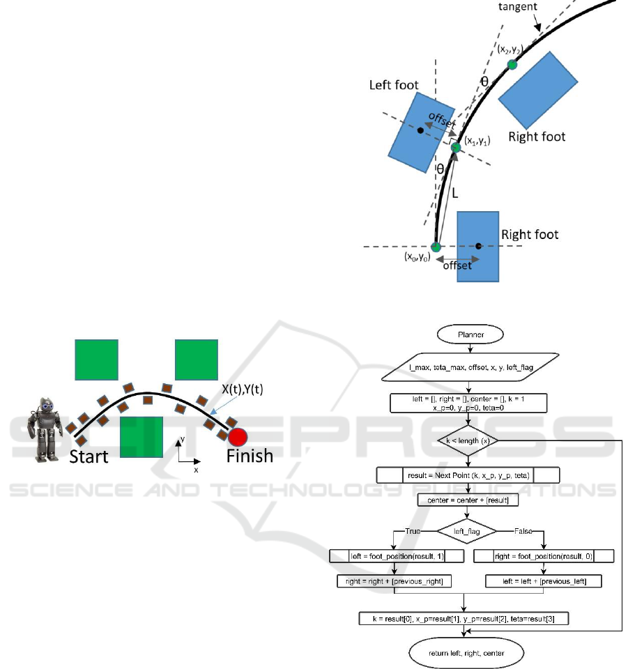
Figure 1: Desired trajectory as an input to foot planner.
Other input parameters for the foot planner are
maximum step length L
max
, maximum rotation angle
for a single step θ
max
, and a distance between foot
center and a closest point on the desired path. These
values are determined by robot’s kinematic
constraints. In Figure 2 step length is L, rotation angle
is θ and distance between feet is offset. Also, it is
required to determine stepping order, i.e. which foot
makes a first step.
The flowcharts of the proposed foot planner
algorithm are presented in Figures 3-4. Here Planner
is a main function that defines step sequence. It
begins with initializing empty arrays for left and right
foot coordinates and a center point (x_p, y_p, teta),
which is located on a desired curve. Let k be the value
of t parameter for point (x_p, y_p). At the beginning
of the curve x_p=0, y_p=0, k=1. In other words, a
desired path always starts from point (0,0) with zero
orientation.
We are moving along the curve by calling
NextPoint function, which calculates next reachable
center point position and orientation. The idea of
Figure 2: Foot planner parameters.
Figure 3: Foot planner flowchart: Planner function (main).
NextPoint function is to decrease step length
gradually from L
max
to 0 by 1 cm until the difference
of orientation angles between the current point and
previous point becomes lower or equal to θ
max
. If step
length decreases to 0, we make only rotation by angle
θ
max
with no change in position. For the known center
point coordinates, foot_position function allows us to
compute positions of left/right foot center. Planner
function stops when we get to the last point of the
curve.
ICINCO 2017 - 14th International Conference on Informatics in Control, Automation and Robotics
418
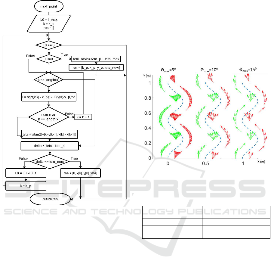
Figure 4: Foot planner flowchart: next_point function.
function foot_position(left,x,y,teta)
if left==true
x=x-offset*cos(teta)
y=y-offset*sin(teta)
else
x=x-offset*cos(teta)
y=y-offset*sin(teta)
return (x, y, teta)
end function
To illustrate the algorithm, let us consider a
sinusoidal curve and run the foot planner for different
maximum rotation angle per step θ
max
. In this case, the
desired path is defined as the following:
1,2..100
0.1 0.1 4 /
0.01
( (100))
t
x cos t
yt
(1)
Simulation results of step planner for θ
max
=5
0
, 10
0
and 15
0
are shown in Figure 6. Here foot positions and
orientations are presented as vectors. When
maximum rotation angle increases, less steps are
required to overcome motion direction change and
complete the path. Table 1 shows number of steps
required to complete the considered path for various
maximum step lengths and rotation angles. The
results highlight stronger dependence of the number
of steps (which is proportional to motion time) on the
rotation angle than on the step length. The direct
correlation between path complexity (convolution
and curvature) and stronger dependency on maximum
rotation angle is obvious.
Figure 5: Foot patterns for different maximum rotation
angles.
Table 1: Number of steps for different parameters of foot
planner so it is centered.
L
max
=10
cm
L
max
=15 cm
L
max
=20 cm
θ
max
=5°
109 steps
101 steps
85 steps
θ
max
=10°
54 steps
54 steps
46 steps
θ
max
=15°
37 steps
37 steps
33 steps
We emphasize that the foot planner is a part of robot
locomotion control. It defines foot positions but does
not determine robot motion between the consequent
steps and does not consider walking stability. The
latter problem is in the focus of the walking engine,
which we describe in the next section. Also, it should
be noted that the process of trajectory generation is
not in the focus of this work. The algorithm
considered in the paper deals with pre-defined
trajectory.
3 WALKING ENGINE
To achieve walking functional, we decompose the
engine into several modules and consider each
module independently. Figure 7 shows all modules
and interaction between them; description of each
module is given below.
Arbitrary Trajectory Foot Planner for Bipedal Walking
419
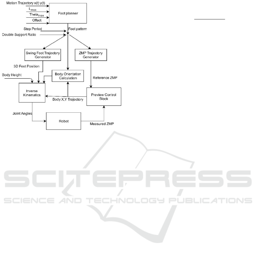
Figure 6: Architecture of walking engine.
3.1 Foot Planner
Foot planner workflow was described in previous
section. We initialize it with a desired path and step
parameters and it returns a set of feet center positions
and orientations along the desired path.
3.2 Swing Foot Trajectory Generator
To generate swing foot trajectory, we need
coordinates and orientation at the beginning and at the
end of the step, which are provided by the foot
planner. The aim of a swing foot trajectory generator
is to obtain time dependant functions for the Cartesian
coordinates x, y, z, θ, where θ corresponds to the foot
rotation around z axis. There are many ways to do it.
For example in (Rai and Tewari) authors use a
polynomial interpolation to obtain a swing leg
trajectory. In (Khusainov et al., 2016) optimal swing
leg trajectory is obtained, taking into account joint
kinematic limits. Here we used trigonometric
functions to build trajectory profile, since they are
simple and can provide zero velocities at contact
moments. Assuming that x
s
and x
f
are coordinates at
start and end of a step calculated by the foot planner,
t
ds
is double support phase time, t
ver
is vertical motion
time, t
0
is step time, x(t) can be written as:
0
0
0
0.5 1 ,
,
,
ds
f s s
ds ver
ds ver
f ve
d
r
ss
tt
x x cos x
t t t
if t t t t
x x if t t t
x x if t t
x
(1)
At the end of the step there is an interval t
ver
with
no motion in x-direction. We introduced this to ensure
strictly vertical motion of the swing foot before
touching the surface and to avoid horizontal
momentum at a contact. Also, it should be noted that
cosine function gives zero velocity values at the
beginning and at the end of motion. Equations for y(t)
and θ(t) are similar, while z(t) coordinate function is
presented as:
0
0.5 1 / ,
0
,
2
d
s
s ds
ds
d
zi
h cos t t t t
i
f
f
tt
z
tt
(2)
where h is a step height. In this work we assume that
the swing foot is always parallel to the ground.
3.3 ZMP Trajectory Generator
A zero-moment point (ZMP) criterion is widely used
as a stability measure in the literature (Vukobratović
and Borovac, 2004) (Lee et al., 2015). To ensure
stable locomotion of the robot, a ZMP point should
lie within supporting polygon, which is the convex
hull of supporting feet area (Vukobratović and
Stepanenko, 1972). Therefore, we can introduce some
reference ZMP trajectory, which always lies within
supporting polygon and compute feasible robot center
of mass (CoM) trajectory so that its ZMP follows the
reference ZMP. Reference ZMP functions for x and y
coordinates, which are the input values for the
controller, are computed from supporting foot center
coordinates, which in turn is calculated from foot
positions and step time. Suppose that robot starts
walking straight ahead with a distance of 20 cm
between the feet. In Figure 8 the reference ZMP is
initially located in the center of right foot (supporting
foot) with coordinate -10 cm, then moves to the center
of left foot with coordinate +10 cm and so on.
Duration of ZMP change is defined by double support
phase time during which both legs are on the ground.
To obtain smooth change of ZMP value we used
cubic spline in a double support phase.
ICINCO 2017 - 14th International Conference on Informatics in Control, Automation and Robotics
420
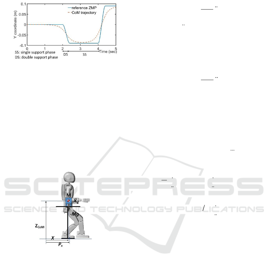
Figure 7: Reference ZMP and CoM trajectory in sagittal
plane.
3.4 Preview Control Block
Preview control block generates CoM trajectory
based on the reference ZMP and active balance
feedback loop. The CoM trajectory can be calculated
by a simple physical model approximating the bipedal
robot dynamics. In our work we use preview control
approach (Kajita et al., 2003) and describe robot
dynamics by inverted pendulum model with
additional constraint on mass height, i.e., three-
dimensional linear inverted pendulum model. There
are several assumptions in this model.
Figure 8: Cart-table model for bipedal locomotion.
The first assumption is that all mass is concentrated
in CoM point, which means that we neglect mass
distribution and suppose that leg’s mass is relatively
small. Although this assumption seems to differ from
reality, effect of leg’s mass can be neglected at a first
approximation, since robot’s trunk is much heavier
than a leg. The second assumption is that CoM
always keeps a constant height. This assumption
significantly simplifies dynamics equations. A cart-
table model, shown in Figure 9, corresponds to the
described model. The cart with mass M moves on a
table with a negligible mass. ZMP coordinate in this
case can be written as:
CoM
x
z
p x x
g
(3)
where
x and x
are CoM coordinate and
acceleration, g is gravity constant,
CoM
z
is CoM
height. For 3D walking we use two cart-table models,
one is for motion in a sagittal plane, the other is for
motion in a frontal plane. Therefore, y coordinate
equation could be written similarly to (4):
CoM
y
z
p y y
g
(4)
If CoM trajectory is given, we can easily calculate
ZMP by using ZMP equations (4) and (5). On the
other hand, for stable motion ZMP should always lie
under a supporting foot. Therefore, we can determine
reference ZMP trajectory knowing supporting foot
coordinates as a function of time. Hence, we have an
inverse problem, where CoM trajectory is calculated
from reference ZMP trajectory.
If we define new variable as
ux
, equation (4)
can be rewritten as dynamical system equation:
0 1 0 0
0 0 1 0
0 0 0 1
10
x CoM
xx
d
x x u
dt
xx
x
p z g x
x
(5)
Then the system can be discretized as
( 1) ( ) ( )
( ) ( )
x k Ax k Bu k
p k Cx k
(6)
where A, B and C matrices are found from (6), k is a
discrete time, x is a state vector, u is a jerk and p is a
ZMP coordinate. (Katayama et al., 1985) presented a
preview control approach that uses a desired future
value of the ZMP coordinates. Authors showed that
the optimal controller for the system with given
reference ZMP p
ref
and previewing N future steps can
be written as:
01
( ) ( ) ( ) ( ) ( )
kN
i x p ref
ij
u k G e k G x k G j p k j
(7)
where G
i
, G
x
and G
p
(j) are gains that are calculated
from controller weights,
ref
e k p k p k
is a
ZMP error. Thus, the preview controller consists of
three terms: the integral error of ZMP, the state
feedback (that is proportional to a current state vector
Arbitrary Trajectory Foot Planner for Bipedal Walking
421
x) and the preview action, which takes into account
future values of the desired ZMP position with the
sum running over N future values. Figure 8 shows
reference ZMP and calculated CoM trajectory in the
frontal plane. Here CoM starts moving before a sharp
change of reference ZMP, which is an effect of
previewing the future reference.
3.5 Body Orientation
Preview controller computes x
CoM
and y
CoM
of the
body with z
CoM
being fixed. There remains 3 DoF for
body orientation definition and 6 DoF undetermined
for swing foot. We put some additional constraints on
the system by setting to zero trunk Y axis rotation,
which means there is no forward-backward
inclination of the trunk. Trunk X axis rotation is
defined by its side inclination. This is done because
of kinematic limits in hip and ankle roll joints.
Suppose that robot stands with parallel feet on the
ground. If we start moving trunk to its right and
remain it upright, at some point we will hit kinematic
limits (marked red in Figure 10).
Figure 9: Body orientation in frontal plane.
Therefore, we should rotate trunk around X axis. To
find the rotation angle we first calculated all possible
trunk rotation angles for a given joint limits and trunk
y coordinate by applying inverse kinematic problem
(see section 3.5). Then we took the middle value of
interval as the best rotation angle. Figure 11 shows
trunk X axis rotation angle as a function of trunk y
coordinate. z
CoM
was set to 0.7 m, maximum hip roll
rotation angles were 0.2 rad for inward and 0.3 rad for
outward rotation. We see piecewise linear uneven
function which can be approximated as:
1.67 , 0.0228
0.8295 0.0228 0.038076,
0.0228
y if y
y
if y
(8)
Function (9) gives us optimal trunk rotation angle
for given CoM y coordinate.
Figure 10: Dependency of optimal rotation angle on CoM y
coordinate.
3.6 Inverse Kinematics
After we have fully defined all 6 DoF for each leg the
next step is to solve inverse kinematics problem for
each leg, i.e. to find joint angles given the position
and orientation of foot and torso.
Figure 11: Leg kinematic scheme.
(Peiper, 1968) showed that if three adjacent joint axes
intersect in a single point, there exists closed-form
solution of the inverse kinematics problem. In our
scheme (Figure 12) we have this condition for hip
joints. Given transformation matrix from global
coordinate system (CS) to torso CS is T
t
and from
global CS to foot CS is T
f
, then we can write
transformation matrix from foot to torso system is
1
ft t f
T TT
. At the same time
1 1 2 2 3 3 4 4 5 5 6 6
( ) ( ) ( ) ( ) ( ) ( )
ft
T T T T T T T
(9)
where
16
...
are joint angles, starting from ankle roll
angle. Since last three rotations do not effect on hip
ICINCO 2017 - 14th International Conference on Informatics in Control, Automation and Robotics
422
joints center position, we firstly find
1 2 3
,,
angles.
After that we substitute calculated angles into (10)
and compare rotation matrices of T
ft
matrix and
product matrix to find remaining three angles. There
are totally eight possible solutions of inverse
kinematics problem so we choose appropriate one.
4 EXPERIMENTAL RESULTS
To demonstrate the proposed algorithm efficiency we
verified its performance with AR-601M bipedal robot
(Figure 13). The robot has totally 41 active degrees of
freedom (DoF), 6 of which are located in each leg:
three joint axes are in the hip, two joints are at the
ankle and one in the knee. The total mass of the robot
is 65 kg and the height is 1442 mm. Further details
about AR-601M are available in (Khusainov et al.,
2015).
Figure 12: Humanoid robot AR601M.
Two trajectories were tested in experimental study.
The first experiment was walking for 2 m distance
along a straight line. The robot’s step length was set
to 15 cm with the step period of 3 seconds. Figure 14
shows foot pattern, CoM trajectory and ZMP
trajectory measured with force sensors. The second
trajectory was defined as sinusoid curve. Step length
was set to 15 cm, maximum rotation angle to 10
0
, and
the step period to 3 seconds and the experimental data
is presented in Figure 15.
Results for average coordinate errors with respect
to the desired goal position are given in Table 2.
These differences were mainly caused by compliance
in actuator joints and errors (and noise) of the sensors.
Yet, these errors are acceptable for the considered
distances and do not overcome 3%. For larger
distances, these errors should be compensated by
external position control, e.g., SLAM methods.
Figure 13: Experimental results: walking on a straight line.
Figure 14: Experimental results: walking along a curve.
Table 2: Average error for position and orientation.
x
cm
y
cm
deg
Straight line
1.5
5
5°
Along a curve
3
3
5°
5 CONCLUSIONS
This paper presents the foot planner algorithm for
biped walking along an arbitrary curve. Together with
the walking engine, it enables the robot to move along
a desired path with acceptable position and
orientation errors. Preview control method was used
as a walking engine balance controller.
The presented biped locomotion approach was
verified with a AR601M robot. Experimental results
illustrated successful performance of the proposed
foot planner method and walking engine architecture.
However, because of accumulated errors of different
nature, for large walking distances our algorithm
would require additional external system to measure
position error, which could provide a feedback loop
and significantly increase position accuracy.
Arbitrary Trajectory Foot Planner for Bipedal Walking
423

ACKNOWLEDGEMENTS
This research has been supported by the grant of
Russian Ministry of Education and Science 2017-14-
576-0053-7882 and Innopolis University.
REFERENCES
Chestnutt, J., Lau, M., Cheung, G., Kuffner, J., Hodgins, J.
and Kanade, T. 'Footstep Planning for the Honda
ASIMO Humanoid'. Proceedings of the 2005 IEEE
International Conference on Robotics and Automation,
18-22 April 2005, 629-634.
Feng, S., Whitman, E., Xinjilefu, X. and Atkeson, C. G.
(2015) 'Optimization‐ based Full Body Control for the
DARPA Robotics Challenge', Journal of Field
Robotics, 32(2), pp. 293-312.
Ha, I., Tamura, Y., Asama, H., Han, J. and Hong, D. W.
'Development of open humanoid platform DARwIn-
OP'. 2011: IEEE, 2178-2181.
Kajita, S., Kanehiro, F., Kaneko, K., Fujiwara, K., Harada,
K., Yokoi, K. and Hirukawa, H. (2003) 'Biped walking
pattern generation by using preview control of zero-
moment point'. Robotics and Automation, 2003.
Proceedings. ICRA '03. IEEE International Conference
on, 14-19 Sept. 2003, 1620-1626 vol.2.
Kajita, S., Morisawa, M., Miura, K., Nakaoka, S. i., Harada,
K., Kaneko, K., Kanehiro, F. and Yokoi, K. 'Biped
walking stabilization based on linear inverted
pendulum tracking'. 2010: IEEE, 4489-4496.
Katayama, T., Ohki, T., Inoue, T. and Kato, T. (1985)
'Design of an optimal controller for a discrete-time
system subject to previewable demand', International
Journal of Control, 41(3), pp. 677-699.
Khusainov, R., Klimchik, A. and Magid, E. 'Swing leg
trajectory optimization for a humanoid robot
locomotion'. Informatics in Control, Automation and
Robotics (ICINCO), 2016 13th International
Conference on.
Khusainov, R., Shimchik, I., Afanasyev, I. and Magid, E.
'Toward a human-like locomotion: Modelling
dynamically stable locomotion of an anthropomorphic
robot in simulink environment'. Informatics in Control,
Automation and Robotics (ICINCO), 2015 12th
International Conference on, 21-23 July 2015, 141-
148.
Lee, D.-W., Lee, M.-J. and Kim, M.-S. 'Whole body
imitation of human motion with humanoid robot via
ZMP stability criterion'. 2015: IEEE, 1003-1006.
Ogura, Y., Aikawa, H., Shimomura, K., Kondo, H.,
Morishima, A., Lim, H.-o. and Takanishi, A. (2006)
'Development of a new humanoid robot WABIAN-2'.
2006: IEEE, 76-81.
Peiper, D. L. (1968) The kinematics of manipulators under
computer control: DTIC Document.
Rai, J. K. and Tewari, R. 'Quintic polynomial trajectory of
biped robot for human-like walking'. 2014: IEEE, 360-
363.
Sakagami, Y., Watanabe, R., Aoyama, C., Matsunaga, S.,
Higaki, N. and Fujimura, K. 'The intelligent ASIMO:
System overview and integration'. 2002: IEEE, 2478-
2483.
Shafii, N., Abdolmaleki, A., Lau, N. and Reis, L. P. (2015)
'Development of an Omnidirectional Walk Engine for
Soccer Humanoid Robots'.
Shamsuddin, S., Ismail, L. I., Yussof, H., Zahari, N. I.,
Bahari, S., Hashim, H. and Jaffar, A. 'Humanoid robot
NAO: Review of control and motion exploration'. 2011:
IEEE, 511-516.
Stasse, O., Davison, A. J., Sellaouti, R. and Yokoi, K. 'Real-
time 3D SLAM for Humanoid Robot considering
Pattern Generator Information'. 2006 IEEE/RSJ
International Conference on Intelligent Robots and
Systems, Oct. 2006, 348-355.
Strom, J., Slavov, G. and Chown, E. (2010)
'Omnidirectional Walking Using ZMP and Preview
Control for the NAO Humanoid Robot', in Baltes, J.,
Lagoudakis, M., Naruse, T. & Ghidary, S. (eds.)
RoboCup 2009: Robot Soccer World Cup XIII Lecture
Notes in Computer Science: Springer Berlin
Heidelberg, pp. 378-389.
Vukobratović, M. and Borovac, B. (2004) 'Zero-moment
point — thirty five years of its life', International
Journal of Humanoid Robotics, 01(01), pp. 157-173.
Vukobratović, M. and Stepanenko, J. (1972) 'On the
stability of anthropomorphic systems', Mathematical
biosciences, 15(1-2), pp. 1-37.
Zhao, Y. and Sentis, L. 'A three dimensional foot placement
planner for locomotion in very rough terrains'. 2012
12th IEEE-RAS International Conference on Humanoid
Robots (Humanoids 2012), Nov. 29 2012-Dec. 1 2012,
726-733.
ICINCO 2017 - 14th International Conference on Informatics in Control, Automation and Robotics
424
