
Modified Spline-based Path Planning for Autonomous Ground Vehicle
Evgeni Magid
1
, Roman Lavrenov
1
and Airat Khasianov
2
1
Intelligent Robotics Department, Higher School of Information Technology and Information Systems,
Kazan Federal University, Kremlyovskaya str. 35, Kazan, Russian Federation
2
Higher School of Information Technology and Information Systems, Kazan Federal University, Kremlyovskaya str. 35,
Kazan, Russian Federation
Keywords:
Path Planning, Voronoi Diagram, Potential Field, Mobile Robot.
Abstract:
Potential function based methods play significant role in global and local path planning. While these methods
are characterized with good reactive behavior and implementation simplicity, they suffer from a well-known
problem of getting stuck in local minima of a navigation function. In this article we propose a modification of
our original spline-based path planning algorithm for a mobile robot navigation, which succeeds to solve local
minima problem and adds additional criteria of start and target points visibility to help optimizing the path
selection. We apply a Voronoi graph based path as an input for iterative multi criteria optimization algorithm.
The algorithm was implemented in Matlab environment and simulation results demonstrate that we succeeded
to overcome our original algorithm pitfalls.
1 INTRODUCTION
Today most robotic applications are targeting for in-
dustrial production speed and quality improvement
as well as for human replacement in various scenar-
ios, which range from social-oriented human-robot
interaction scenarios (Pipe et al., 2014) to danger-
ous for a human urban search and rescue scenar-
ios (Magid et al., 2011). The later scenarios may in-
clude indoor and outdoor environments and require
good performance in autonomous navigation within
unknown environments (Indelman et al., 2015), abil-
ity to deal with computational complexity of simul-
taneous localization and mapping (SLAM) (Buyval
et al., 2016), capabilities of negotiation and collab-
oration (Panov and Yakovlev, 2017) with other robots
within a team (Rosenfeld et al., 2015) or swarm con-
trol (Ronzhin et al., 2016) and other functionality.
Path planning is probably the most essential part
of autonomous navigation for a mobile robot, which
is responsible for providing a collision-free path be-
tween initial and goal positions of the robot. A good
path planning algorithm should guarantee its com-
pleteness, i.e. the robot should reach its goal position
or conclude explicitly that a path, which could con-
nect the start and the goal positions, does not exist.
The completeness property is by default incorporated
into all global path planning methods, but for local
path planning in order to satisfy this property vari-
ous strategies are applied. The classical global path
planning approach, which is referred as piano movers
problem, utilizes complete a priori knowledge about
environment: a robot is aware of its own shape, ini-
tial and goal position and orientation, and a set of 2D
or 3D environment obstacles, where each obstacle in-
formation includes precisely defined shape, position,
orientation in space and other task-related data (e.g.,
texture or traversability index (Seraji, 1999)). Next,
the robot searches for a continuous path from the ini-
tial position to the goal position, while negotiating
with static obstacles of the environment along its way.
In order to simplify the procedures, often the concept
of multi-dimensional configuration space (Latombe,
2012) is applied for the planning. In such settings,
the path planning operation becomes an off-line one-
time operation since a complete knowledge about the
environment is available in advance. This allows op-
timizing a solution with regard to various criteria in
order to obtain an optimal or at least sub-optimal path
relatively to these criteria. The path search algorithm
should consider such qualities as ability to generate a
collision free path, time and space complexity, ability
to discover a path if it does exist, efficient computa-
tional scheme, and the later is actually the main diffi-
culty of the piano movers approach. Yet, in real world
scenario the robot does not possess a complete knowl-
edge about environment - except some very limited or
artificial application cases. For this reason the robot
132
Magid, E., Lavrenov, R. and Khasianov, A.
Modified Spline-based Path Planning for Autonomous Ground Vehicle.
DOI: 10.5220/0006442601320141
In Proceedings of the 14th International Conference on Informatics in Control, Automation and Robotics (ICINCO 2017) - Volume 2, pages 132-141
ISBN: Not Available
Copyright © 2017 by SCITEPRESS – Science and Technology Publications, Lda. All rights reserved
should continuously collects sensory data from its po-
tentially dynamic environment and plan the path ac-
cordingly, which requires a reasonable combination
of local and global methods of path planning.
When a robot uses incoming sensory data to create
a global world map as it traverses the environment, we
refer to such approach as global sensor-based plan-
ning. Next, the created map is used for path plan-
ning. Main weakness of global sensor-based plan-
ning approach is a significant computational burden
on the robot while creating and maintaining a global
model as well as excessive memory requirements in
order to store the model and the large amount of sen-
sory information, which is associated with the model.
Purely local path-planners avoid these issues by uti-
lizing only local sensory information; this allows to
reactively negotiate environmental obstacles but does
not guarantee global convergence. This way, in order
to provide a superior performance, a well-balanced
integration of global and local path-planners is essen-
tial.
A classical and popular path planning ap-
proach applies potential field method (Tang et al.,
2010), (Khatib and Siciliano, 2016), which is based
on an artificial potential field concept that marks a
goal position as an attractive pole and obstacles are
represented with repulsive surfaces. Then a robot pur-
sues the potential gradient in the direction of its min-
imum. Potentials are generated either at a global or
a local level and this is a matter of available envi-
ronmental information (Andrews and Hogan, 1983).
Potential field methods gained their popularity due
to algorithm simplicity and a capability of fast re-
active avoidance of mobile and stationary obstacles.
However, potential field methods are typically fea-
tured with such drawbacks as path oscillations for
certain configurations of obstacles (e.g., narrow pas-
sages) and local minima problem, which captures a
robot in a potential function local valley and requires
special escape procedure in order to proceed (e.g., se-
quence of random steps in arbitrary direction).
In our previous research we had proposed a path
planning spline-based algorithm for a car-like mobile
robot within a well-known environment (Magid et al.,
2006). It uses potential field method for obstacle
collision avoidance to provide a locally sub-optimal
path with regard to path length, path smoothness and
safety optimization criteria. While a typical path-
planning algorithm applies final smoothing of a path
at the last stages only (Fleury et al., 1995), (Elban-
hawi et al., 2015), our algorithm special feature is the
smoothness criterion integration into path optimiza-
tion from the first stage of the algorithm. Other crite-
ria (path length and safety) played secondary role in
optimization procedure and thus collision-free but not
sufficiently smooth path was treated as a low quality
one. In order to improve the original algorithm per-
formance, to add flexibility for path optimization and
a possibility for a fast dynamic replanning in a case
the initially off-line selected path becomes unavail-
able, we integrate Voronoi Diagram approach into our
algorithm (Choset and Burdick, 1995).
The rest of the paper is organized as follows. Sec-
tion 2 briefly describes our previous research within
spline-based path planning. In section 3 we present
new criteria that improve the algorithm performance
and add more flexibility for the user while select-
ing path evaluation measures. Section 4 presents
our modification of the spline-based algorithm, which
successfully overcomes the weaknesses of the initial
approach. Section 5 demonstrates the original and
the new algorithm trial examples, where the new al-
gorithm shows successful solution of the original al-
gorithm failures. Section 6 discusses our future work.
Finally, we conclude in Section 7.
2 SPLINE-BASED ROBOT
NAVIGATION WITH ORIGINAL
POTENTIAL FIELD APPROACH
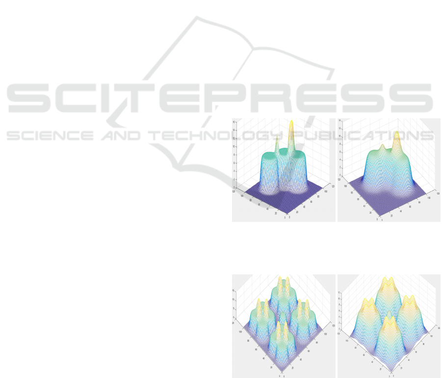
Figure 1: Repulsive potential function of eq. 1 for α = 0.5
(left) and α = 0.2 (right) that corresponds to the obstacles
in Figure 4.
Figure 2: Repulsive potential function of eq. 1 for α = 0.5
(left) and α = 0.2 (right) that corresponds to the obstacles
in Figure 5.
Modified Spline-based Path Planning for Autonomous Ground Vehicle
133

The spline-based method, proposed by Magid
et.al. about a decade ago (Magid et al., 2006) navi-
gates a car-like robot in a planar known environment
populated with static obstacles. The algorithm is con-
sidering an omnidirectional circle-shape robot which
reduces a search space by one dimension (an orienta-
tion) and all further actions are performed for a point
robot in a 2D configuration space. An obstacle is pre-
sented with a set of intersecting circles of different
sizes and each set may contain just a single circle or a
finite number of circles. The idea behind such restric-
tion is based on the assertion that any arbitrary ob-
stacle could be well-approximated with a finite set of
circles. Next, given a complete information about the
environment, a start and a target positions of the robot,
the robot searches for a collision-free path which is
guided by a pre-determined cost function. The de-
tails of the algorithm could be found in (Magid et al.,
2006), while in this section we briefly describe the se-
lected cost functions and overview the algorithm, and
demonstrate a successful example of its execution and
two failing examples. Finally, we explain the origins
of these failures in subsection 2.3 and further suggest
its modification in Section 4.
2.1 Cost Function
To provide the collision free path, a repulsive poten-
tial function is featured with a high value inside an
obstacle and on its border and a small value within
free space. This way, high value of the potential
function in the obstacle’s centre pushes all points of
a path outside in order to minimize path cost during
local optimization procedure. The potential field be-
gins to drastically change (decline) on obstacle’s bor-
der, keeps decreasing with distance as a point moves
away from the border and becomes zero rather fast in
a close vicinity of the obstacle. Assuming the robot’s
position at q(t) = (x(t), y(t)) for a time-stamp t, a con-
tribution of a single circle (where the circle is a part of
an obstacle) repulsive potential to the global potential
function is defined with the following equation:
U
rep
(q) = 1+tanh(α(ρ−
q
(x(t) − x)
2
+ (y(t) − y)
2
))
(1)
where ρ is the radius of the obstacle with the centre at
(x, y) and α is an empirically defined parameter that is
responsible for pushing a path outside of an obstacle.
Figure 1 demonstrates the examples of two different
selections of α parameter (α = 0.5 in the left sub-
figure and α = 0.2 in the right) for the environment
with a single obstacle that is formed by three inter-
secting circles, shown in Figure 4. Similarly, Figure 2
demonstrates the examples of α = 0.5 (in the left sub-
figure) and α = 0.2 (in the right sub-figure) for the en-
vironment with one circular obstacle in the centre and
four symmetrical complicated concave obstacles (that
are formed by four intersecting circles each), which
correspond to the map in Figure 5. In the later ex-
ample, potential function has clear peaks at the circle
intersections.
Topology T (q) is a function that takes into an ac-
count all N obstacles of the environment and their in-
fluence on the robot along the whole path, which is
defined as a parametric function within [0,1]:
T (q) =
N−1
∑
j=0
Z
1
t=0
U
j
rep
(q) · δl(t) · dt (2)
where δl(t) is simply a length of a segment:
δl(t) =
q
(x
0
(t))
2
+ (y
0
(t))
2
(3)
A function for smoothness property of the path
is referred as Roughness R(q) and is also integrated
along the path:
R(q) =
s
Z
1
t=0
(x
00
(t))
2
+ (y
00
(t))
2
dt (4)
A function that accounts for the path length L(q) sim-
ply sums up the lengths of all path segments:
L(q) =
Z
1
t=0
δl(t)· dt (5)
Then, the final path cost function accumulates all the
three above components:
F(q) = γ
1
T (q) + γ
2
R(q) + γ
3
L(q), (6)
where γ
i=1..3
are the weight factors that set an influ-
ence of the corresponding component on a total cost
of the path. In particular obstacle penalty influence
component is empirically defined as γ
1
=
β
2
, where β
ranges over a predefined array, which correlates with
array of α parameters from eq.1 (Magid, 2006).
2.2 The Algorithm
The original algorithm of spline-based path planning
works iteratively, beginning with start point S and tar-
get point T , and utilizes the environment obstacles as
its input data. An initial path is suggested as a straight
line between points S and T , which serves as a first
spline-based path and its spline is defined with three
points: S, T and a equidistant point that lies on the
straight line between them. Equation 6 sets a current
path cost, which is further optimized with Nelder-
Mead Simplex Method (Lagarias et al., 1998) in or-
der to minimize the path cost. A resulting better path
serves as an initial guess for the next iteration.
ICINCO 2017 - 14th International Conference on Informatics in Control, Automation and Robotics
134
The optimization procedure operates only with
those points of the path, which define its spline, while
path evaluation accounts for all points of the path.
The path-defining spline is rebuilt at each iteration us-
ing information from a previous stage, increasing the
number of spline’s points by one and adjusting pa-
rameters of the target cost function. Once the path
is free of obstacles, a few more iterations are con-
ducted in order to improve the resulting path locally.
The algorithm terminates if iteration count exceeds a
user-defined limit or if a new iteration does not suc-
ceed to improve a previous one, while increasing the
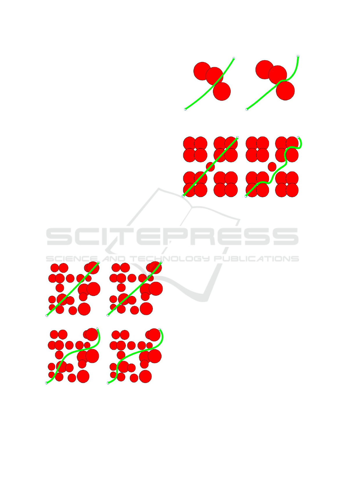
spline complexity. Figure 3 demonstrates an example
of the algorithm successful execution within a simple
convex obstacles environment that resembles a plaza
with ideal geometrical placement of equal columns or
flowerbeds (a view from the above): the initial path is
an optimized with regard to eq.6 spline with a single
via point between S and T (Figure 3a); after four iter-
ations the spline has four via points but still collides
with the obstacles (Figure 3b); after seven iterations
the 7-via-points-spline could be already applied for
navigation (Figure 3c), but two more iterations suc-
ceed to improve path’s length and smoothness prop-
erties (Figure 3d, 9th iteration); further increase of via
points number does not provide any improvement of
the path. It took 9 minutes to obtain the final path
after 9 iterations of the algorithm.
(a) (b)
(c) (d)
Figure 3: Simple convex obstacles: (a) the initial state, (b) 4
iterations, (c) 7 iterations, (d) the final path after 9 iterations.
Figure 4: Simple concave obstacle: the first iteration path
(left) and the final path after 12 iterations (right).
Figure 5: Two complicated concave obstacles: the first iter-
ation path (left) and the final path after 17 iterations (right).
2.3 Drawbacks of the Approach
The original spline-based method succeeds to obtain
a collision free smooth path for any complexity of the
environment if each obstacle is approximated with a
single circle under the condition of non-intersecting
obstacles and some minimal distance between the ob-
stacles, which would provide a safety gap for the
moving along a path mobile robot. In this case, since
the potential function diminishes rapidly as we move
away from the obstacle boundary, we could neglect
the probability of getting stuck in a local minima.
However, when the obstacles are to be approximated
with a number of intersecting circles, the intersections
introduce potential field local maxima. Moreover, if
in such settings an initial spline passes through in-
tersection of several obstacles, the cost function F(q)
concentrates on pushing the spline out of intersection
area that forms a local maximum; upon successful
pushing out, a further solution often gets stuck in a lo-
cal minima and a next iteration spline can not ”jump
over” some obstacle components due to a local nature
of the optimization process. Figure 4 presents a sim-
ple case of an obstacle that is formed by three inter-
secting circles and the corresponding potential field is
presented in Figure 1; after 12 iterations the algorithm
stops as no further improvements are possible - while
a spline succeeds to optimize the path locally so that
it avoids a local maximum, it is still stuck at a local
minimum and the resulting path could not be used for
Modified Spline-based Path Planning for Autonomous Ground Vehicle
135

navigation due to obstacle collision. Figure 5 demon-
strates an example with five complicated concave ob-
stacles and a narrow pass in between. Due to multi-
ple intersecting circles, which generate their own lo-
cal repulsive potentials, the corresponding global field
conceals the pass (Figure 2) and permits only a local
optimization of the path. The local optimization suc-
cessfully avoids local maxima, but even after 37 iter-
ations that continued for 44 minutes, the final path is
still occluded with obstacles and thus useless for nav-
igation.
3 INTEGRATING ADDITIONAL
OPTIMIZATION CRITERIA
The original spline-based algorithm uses just three
criteria within cost function (eq. 6): topology, rough-
ness and length of path. In this section we introduce
two new additional criteria - start and target point vis-
ibility time - and explore their influence on the result-
ing path. Point visibility time refers to the path length
where the robot keeps the start point (or target point
respectively) within its direct line of sight without any
obstacle occlusions.
These two criteria are important if a robot needs to
maximize the time of a direct visual or radio contact
with a monitoring device or a router, which supports
path planning, localization or any other functionality
of the robot. The criterion should consider the ra-
tio of visible and invisible from the start (or target)
points segments of a path. Thus, we need to maxi-
mize the time when the robot is visible from the start
point while following the selected path before it dis-
appears behind some obstacle for the first time. In
other words, we minimize the time (which is actually
measured as a length of the path assuming a constant
speed of the robot - in our future work we also extend
this to the cases of varying speed along the path) after
the robot becomes occluded for the first time, which
we refer as invisibility of the start point S:
I
S
= 1 − lim
δt,δl(t)→0
∑
u
t=0
dist(A(t), A(t +δt))
R
1
t=0
δl(t)· dt
(7)
such that
∀t ∈ [0, u + δt] : [A(t), S] ∩ (∪
N
j=1
Obs
j
) =
/
0 (8)
where the numerator of the fraction in Eq. 7 reflects
the path length of a visible from the start position S
segment and the denominator of the fraction reflects
path length from Eq. 5. A(t) is a position of the robot
at timestamp t, and short segments of the path that
were travelled between timestamp t and t + δt, which
are denoted by dist(A(t), A(t + δt), are accumulated.
Eq. 8 describes the visibility property, which means
that a straight segment [A(t), S] does not intersect any
obstacle Obs
j
where j = 1..N and N is a number of
obstacles in the environment. Thus, the last visible
point from the start point while the robot follows the
selected path before disappearing behind an obstacle
for the first time is described with A(u + δt). Simi-
larly, we describe the criterion that shows the ratio of
visible and invisible from the target point segments
of a path, which we refer as invisibility of the target
point T :
I
T
= 1 − lim
δt,δl(t)→0
∑
1−δt
t=w
dist(A(t), A(t +δt))
R
1
t=0
δl(t)· dt
(9)
such that
∀t ∈ [w, 1] : [A(t), T ] ∩ (∪
N
j=1
Obs
j
) =
/
0 (10)
Eq. 9 and 10 describe the first point A(w) of a path
segment [A(w), A(1) = T ] that marks the beginning of
the last segment of the path which is featured by a
guaranteed constant visual contact between the robot
and the target position T while the robot follows the
selected path.
The cost function that combines all five criteria is
defined as follows:
F(q) = γ
1
T (q)+γ
2
R(q)+γ
3
L(q)+γ
4
I
S
+γ
5
I
T
, (11)
where γ
4
and γ
5
are the weight factors that set the line-
of-sight criteria influence on a total cost of the path
for start S and target T points respectively. Figure 6
demonstrates the two criteria influence on the path
in the vicinity of start and target points: while with
γ
4
=10 and γ
5
=10 these criteria do not contribute any
significant influence (left sub-figure), with γ
4
=20 and
γ
5
=20 the path changes are clearly visible, especially
as the robot approaches the target position (right sub-
figure); other parameters are defined as γ
1
=1, γ
2
=1,
and γ
3
=0.5 for both cases (both sub-figures).
As the path optimization with regard to Eq. 11 is
performed only locally, the influence of the two addi-
tional parameters is also local. As a part of our future
work we plan to apply the optimization at a global
scale, which will allow the path to vary different ho-
motopy sets in order to satisfy and emphasize a par-
ticular user-defined criterion influence.
4 VORONOI DIAGRAM BASED
SOLUTION
We recognize that the local nature of the optimiza-
tion procedure creates a strong dependence of algo-
rithm success or failure on initial spline. In order to
ICINCO 2017 - 14th International Conference on Informatics in Control, Automation and Robotics
136
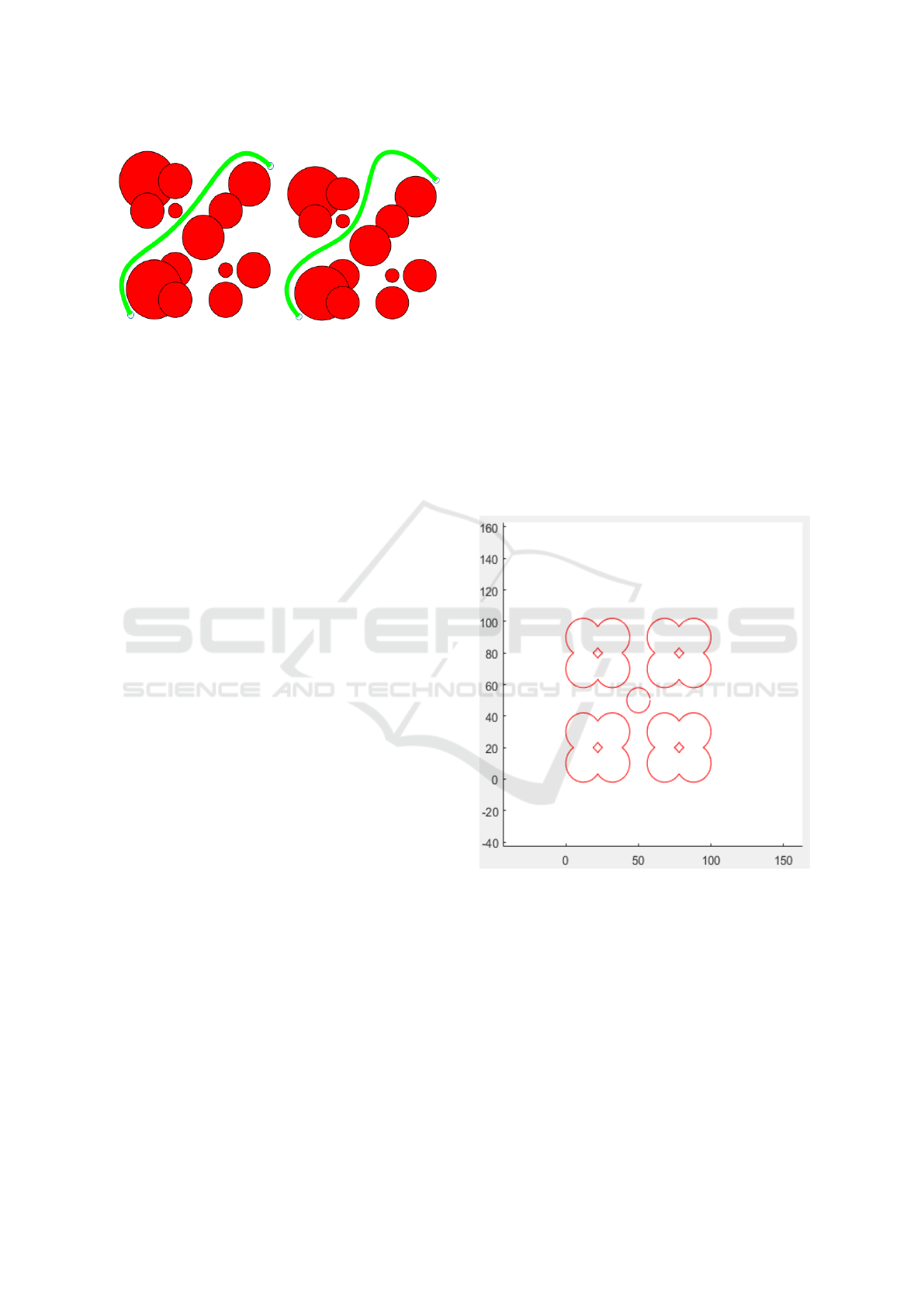
Figure 6: Start and target points visibility time influence
on the path quality: γ
4
=10, γ
5
=10 (left) and γ
4
=20, γ
5
=20
(right).
provide a good initial spline that could be further im-
proved locally with regard to user selection of the cost
weights, we apply Voronoi Diagram approach (Toth
et al., 2004). This helps to avoid the spline seizing at
local minima.
Assuming the above definition of environment ob-
stacles and potential field, prior to Voronoi graph con-
struction, the two following steps are performed in or-
der to prepare the environment:
1. Register obstacles by grouping intersecting cir-
cles together in order to form a single obstacle. Ini-
tially, every circle is marked as idle and has its own
index i = 1..M, where M is a finite number of circles
within the environment. We start from an arbitrarily
circle, assign it to obstacle O
1
and mark as an acti-
vated one. Next, we iteratively grow O
1
by search-
ing for all idle circles that intersect with O
1
, assign
them to obstacle O
1
and mark as activated as well.
The iterative growth of O
1
continues until no more
idle circles that intersect O
1
are left in the environ-
ment. When the iterative growth of O
1
is completed
but there are still idle obstacles available, we select
another arbitrarily idle circle, assign it to obstacle O
2
and repeat the growth procedure. Obstacles registra-
tion is completed when all circles of the environment
become activated. For example, there are five obsta-
cles that are formed by groups of circles in Figure 7
and twelve obstacles in Figure 8. While performing
the registration, each pair of intersecting circles i and
j provides their intersection point ω
i j
in a case there
is a single joint point (i.e., boundary touch) and a pair
of points ω
i j
, ω
ji
in a case of joint two points (i.e.,
boundary intersection).
2. Find outer and inner boundaries of each obsta-
cle of set Obst = {O
1
, O
2
, ..., O
k
}, where k is a num-
ber of compound obstacle within the environment.
Starting from an arbitrary circle within O
1
obstacle,
boundaries of all circles that belong to O
1
are split
into short segments of length σ, merged via intersec-
tion points ω
i j
(or ω
ji
) and labelled. Parameter σ is
predefined in advance and correlates with a radius of a
smallest circle of the environment in order to further
match a shortest polygonal edge of contours. Thus,
during the procedure, two segments receive the same
label if there exists a continuous path between them,
which is built of boundary segments. This procedure
is repeated for each obstacle and upon its completion
we receive a set of obstacles’ boundaries. If the size
of the latter set exceeds the size of Obst, it points out a
presence of inner boundaries that were formed by in-
ternal contours. To get rid of such contours, for each
particular obstacle O
i
we encapsulated every contour
of O
i
into a convex hull, verify which of the result-
ing contours forms outer boundary of O
i
and remove
the rest. For example, this procedure has successfully
removed four tiny diamond-shape internal contours
inside complicated obstacles of environment in Fig-
ure 7. Finally, we obtain several non-convex poly-
gons, one for each obstacle within Obst, and tightly
encapsulate them into a square map.
Figure 7: External contours of group of obstacles.
Next, Voronoi graph is constructed as follows, based
on a classical brushfire approach (Choset, 2005):
1. Parse free space with rays that originate from ob-
stacles’ edges and square map boundary. Figure 8
(the bottom image) demonstrates an example of
Voronoi graph construction for the environment in
the top image of the figure. Thick blue lines de-
pict borders of obstacles of Obst set and thin blue
lines are emerging outwards and inwards rays.
2. Calculate rays intersection points and connect
them with segments for neighbouring ray. These
Modified Spline-based Path Planning for Autonomous Ground Vehicle
137
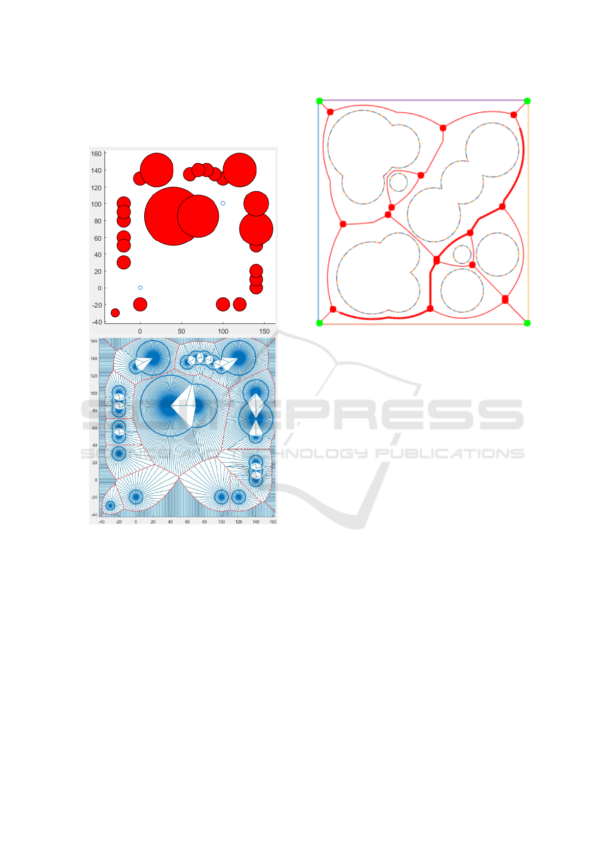
segments are equidistant to nearest obstacles, and
all together form Voronoi graph, which is depicted
with a thin red line in Figure 8 (the bottom image)
Figure 8: Environment with obstacles (top) and Voronoi
graph building procedure (bottom).
Upon obtaining Voronoi graph V G, we select nearest
to start position S and target position T points (S
0
and
T
0
respectively) within V G so that segments [S, S
0
] and
[T, T
0
] lie in the free space of the environment. Next,
shortest paths between S
0
and T
0
are found within
V G applying Dijkstra algorithm (Dijkstra, 1959); they
are depicted with thick red lines in Figure 9). Any
path (S, T ) on Voronoi graph V G is guaranteed to be
collision free and maximally safe with regard to dis-
tance from obstacle boundaries, and thus could pro-
vide a good initial spline for the original spline-based
method (Magid et al., 2006).
If we use points S, T and Voronoi graph V G nodes
(thick red points on Figure 9), which are a part of
some selected path (S, T ), in a role of via points for
Figure 9: The obtained Voronoi graph and a path within the
graph.
initial spline, such sparse selection may fail to guar-
antee a good start of the spline-based method. On the
opposite, selecting every point of some selected path
(S, T ) provides us with a dense and excess amount of
via points. Our trade-off solution that uses a small
set of special points of V G (that belong to the path)
utilizes only via points that would properly charac-
terize path’s features yet avoid redundant complexity
of a spline. At a first step, S is selected as a active
point and a farthest visible from S point of the path,
V P
1
, is calculated. S is added to {L}, while V P
1
re-
ceives a status of a next active point and again a far-
thest visible from V P
1
point of the path, V P
2
, is cal-
culated. V P
1
is added to {L}, V P
2
becomes a next ac-
tive point and the process continues until target point
T becomes visible. Here, point VP
i+1
is visible from
point V P
i
if they could be connected with a straight
segment that does not collide with any obstacle of the
environment. After the process finishes, the points of
{L} are utilized as via points for initial spline of the
spline-based method (Magid et al., 2006).
5 SIMULATIONS
In order to verify our approach the new smart spline-
based algorithm was implemented in Matlab environ-
ment and an exhaustive set of simulations was per-
formed. Particular attention was paid to the cases
where the original algorithm failed (Magid et al.,
2006). The cost function of Eq. 11 was applied with
ICINCO 2017 - 14th International Conference on Informatics in Control, Automation and Robotics
138
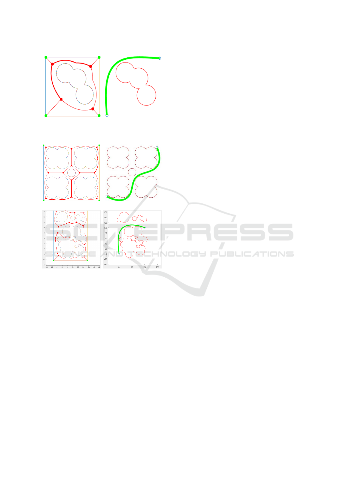
Figure 10: Path planning results: path on Voronoi graph
(left) and the corresponding spline-based optimal path
(right).
(a) (b)
(c) (d)
Figure 11: Path planning results: paths within Voronoi
graph (a,c) and the corresponding spline-based optimal
paths (b,d).
the following empirical parameter selection: γ
1
=1,
γ
2
=1, γ
3
=0.5, γ
4
=5, and γ
5
=5. The algorithm suc-
ceeded to provide collision-free paths in all cases,
which was a natural consequence of applying initial
Voronoi-based path as an input of our iterative algo-
rithm at the first stage of the procedure.
Figure 11 demonstrates two environments, where
the original spline-based algorithm had failed (e.g.,
the example in sub-figure (b) corresponds to Fig-
ure 5). Voronoi graph provides us with a safe path
without obstacle collision or may barely touching the
obstacle boundaries in a case of very narrow passages
between distinct obstacles (of configuration space).
Therefore, this good initial path ensures that the mod-
ified spline-based algorithm would calculate a final
path within a significantly smaller number of itera-
tions. Our preliminary concern about the time com-
plexity of Voronoi graph construction turned out to be
obsolete as the simulations empirically demonstrated
that Voronoi graph calculations take acceptably small
amount of time (at least for our reasonably simple
cases, while more simulations in complicated large-
size environments are scheduled as a part of the future
work).
For example, for the environment of Figure 11(a)
the Voronoi-based initial path calculation took only 2
seconds, while for Figure 11(c) - 6 seconds. The total
running time of the new algorithm decreased in three
times in average with regard to the original algorithm.
This way, the final path of Figure 11(b) was calcu-
lated in just 2 iterations within 2.5 minutes in Matlab,
while the original spline-based algorithm had spent 17
iterations and 44 minutes to conclude on its failure to
provide an acceptable path from start to target point.
Similarly, the original algorithm required 9 iterations
and 15 minutes to provide a good path within Figure 3
environment, while the new algorithm required 5 it-
erations and 4 minutes. In another case of Figure 4
the original algorithm failed to find a path, while a
Voronoi-based algorithm successfully completed the
task within 3 iteration and 2 minutes (Figure 10).
6 DISCUSSION AND FUTURE
WORK
The computation time in minutes per iteration of our
currently implemented spline-based algorithm in its
Matlab prototype is an obstacle for dynamical on-line
planning with changing or dynamic environments in
practical applications. However, we emphasize that a
full-scale Voronoi graph construction and path plan-
ning are performed off-line before a search and res-
cue mission starts in order to select an initial path
of the vehicle. Then, as the vehicle discovers new
or dynamical obstacles on its way, the graph could
be rebuilt only locally (e.g., using techniques similar
to (Kalra et al., 2009) or creating a local virtual gener-
alized Voronoi graph (Choset et al., 2000)) and local
replanning is performed. Local replanning, as well as
implementation speed up and optimization, are parts
of our ongoing and future work. We strongly believe
that C++ implementation will significantly increase
all computations.
The selection of gamma
n
(n=1, , 5) coefficients in
equation (11) is very important for a successful path
planning in practical applications. Currently, the se-
lection is performed empirically, which in our opinion
is a rather weak point of the algorithm. As one of the
possible further extensions of this work, a separate
project for theoretical or comparative approach with
Modified Spline-based Path Planning for Autonomous Ground Vehicle
139
exhaustive simulations and further analysis of the ob-
tained data would be of a great value for proper selec-
tion of these parameters.
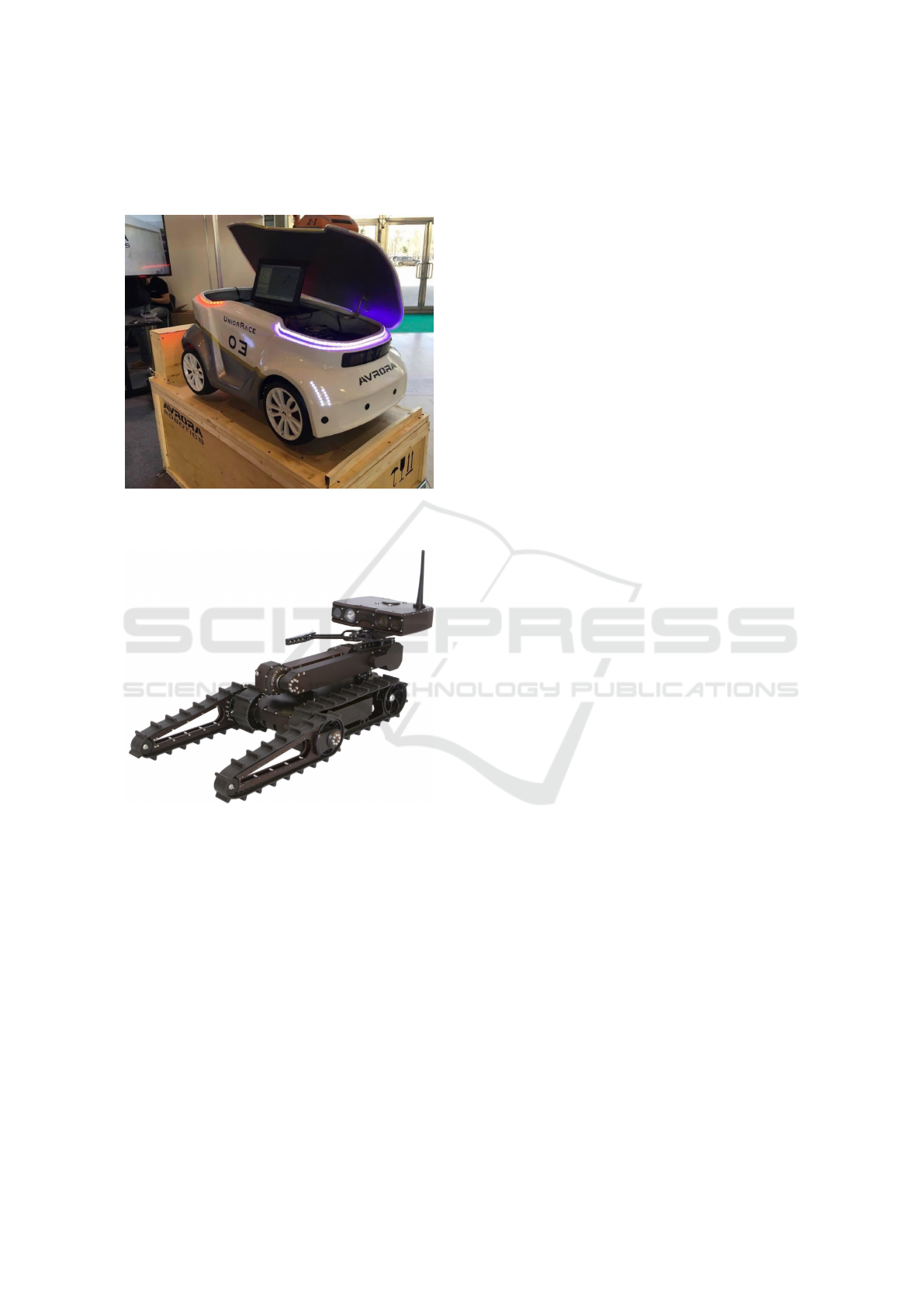
Figure 12: Unior robot, courtesy of Avrora robotics com-
pany, Russia.
Figure 13: Servosila Engineer mobile robot, courtesy of
Servosila company, Russia.
As a part of our future work we plan to introduce
some new parameters of cost function, including
varying speed of the robot along the path. The al-
gorithm will be tested in large-size environments in
order to verify the acceptability of the Voronoi-graph
construction time for more complicated cases. We
would like to apply optimization procedure at a global
scale, which will allow the path to vary different ho-
motopy sets in order to satisfy and emphasize a par-
ticular user-defined criterion influence. Moreover,
we consider extending the algorithm for 3D envi-
ronment and adding new parameters of cost function
that are associated with 3D surfaces. The algorithm
will be bundled into a ROS package with C++ im-
plementation and further verified with real navigation
of a heterogeneous robotic team operating in an ur-
ban search and rescue scenario. Real experimenta-
tion in real world, both static and dynamic, are op-
timistically scheduled for 2018 and will be executed
utilizing Unior car-type mobile robots 12 and a group
of DJI Phantom quadcopters. Additional testing will
be performed with our crawler ”Servosila Engineer”
mobile robot 13, in ROS-Gazebo simulation (Sokolov
et al., 2016), as well as with a real hardware in order
evaluate the applicability of the algorithm for crawler-
type robots. In addition, it will be interesting to com-
pare our solution with the adaptive elliptic trajecto-
ries for smooth and safe mobile robot navigation ap-
proach (Adouane et al., 2011) and trying another rep-
resentation of complex shaped obstacles in harmonic
potential fields (Daily and Bevly, 2008).
7 CONCLUSIONS
A typical difficulty of path planning with potential
function methods is getting stuck in local minima of a
navigation function. In this paper we have presented
a combined method for calculating a smooth and safe
path for mobile robot in static planar environment.
The introduced modifications of our original spline-
based path planning algorithm for a mobile robot nav-
igation helped avoiding local minima problem and
added more flexibility for path optimization. We so-
phisticated the cost function by introducing additional
criteria that maximized the time of keeping the robot
within direct line of sight from start and target points
while the robot follows the path. We also integrated a
Voronoi graph approach into the algorithm in order to
produce a good starting path for iterative spline-based
optimization. The new smart spline-based method al-
gorithm was implemented in Matlab environment and
its results were explicitly compared with our origi-
nal algorithm. The new approach requires less opti-
mization iterations that the original algorithm due to
a smart selection of an initial spline. While the origi-
nal algorithm fails to find an existing path in compli-
cated environments with multiple concave obstacles,
its smart version was successful in all simulated tests
because of the Voronoi graph approach nature.
ACKNOWLEDGEMENTS
This work was partially supported by the Russian
Foundation for Basic Research (RFBR) and Ministry
of Science Technology & Space State of Israel (joint
project ID 15-57-06010). Part of the work was per-
formed according to the Russian Government Pro-
ICINCO 2017 - 14th International Conference on Informatics in Control, Automation and Robotics
140

gram of Competitive Growth of Kazan Federal Uni-
versity.
REFERENCES
Adouane, L., Benzerrouk, A., and Martinet, P. (2011). Mo-
bile robot navigation in cluttered environment using
reactive elliptic trajectories. IFAC Proceedings Vol-
umes, 44(1):13801–13806.
Andrews, J. R. and Hogan, N. (1983). Impedance control
as a framework for implementing obstacle avoidance
in a manipulator. Master’s thesis, M. I. T., Dept. of
Mechanical Engineering.
Buyval, A., Afanasyev, I., and Magid, E. (2016). Compar-
ative analysis of ros-based monocular slam methods
for indoor navigation. 9th International Conference
on Machine Vision (ICMV), Nice, France.
Choset, H. and Burdick, J. (1995). Sensor based planning.
i. the generalized voronoi graph. In Robotics and
Automation, 1995. Proceedings., 1995 IEEE Interna-
tional Conference on, volume 2, pages 1649–1655.
IEEE.
Choset, H., Walker, S., Eiamsa-Ard, K., and Burdick,
J. (2000). Sensor-based exploration: Incremental
construction of the hierarchical generalized voronoi
graph. The International Journal of Robotics Re-
search, 19(2):126–148.
Choset, H. M. (2005). Principles of robot motion: theory,
algorithms, and implementation. MIT press.
Daily, R. and Bevly, D. M. (2008). Harmonic potential field
path planning for high speed vehicles. In American
Control Conference, 2008, pages 4609–4614. IEEE.
Dijkstra, E. W. (1959). A note on two problems in connex-
ion with graphs. Numerische mathematik, 1(1):269–
271.
Elbanhawi, M., Simic, M., and Jazar, R. N. (2015). Con-
tinuous path smoothing for car-like robots using b-
spline curves. Journal of Intelligent & Robotic Sys-
tems, 80(1):23–56.
Fleury, S., Soueres, P., Laumond, J.-P., and Chatila, R.
(1995). Primitives for smoothing mobile robot trajec-
tories. IEEE transactions on robotics and automation,
11(3):441–448.
Indelman, V., Carlone, L., and Dellaert, F. (2015). Planning
in the continuous domain: A generalized belief space
approach for autonomous navigation in unknown en-
vironments. The International Journal of Robotics Re-
search, 34(7):849–882.
Kalra, N., Ferguson, D., and Stentz, A. (2009). Incremen-
tal reconstruction of generalized voronoi diagrams on
grids. Robotics and Autonomous Systems, 57(2):123–
128.
Khatib, O. and Siciliano, B. (2016). Springer handbook of
robotics. Springer.
Lagarias, J. C., Reeds, J. A., Wright, M. H., and Wright,
P. E. (1998). Convergence properties of the nelder–
mead simplex method in low dimensions. SIAM Jour-
nal on optimization, 9(1):112–147.
Latombe, J.-C. (2012). Robot motion planning, volume 124.
Springer Science & Business Media.
Magid, E. (2006). Sensor-based robot navigation. Master’s
thesis, Technion - Israel Institute of Technology.
Magid, E., Keren, D., Rivlin, E., and Yavneh, I. (2006).
Spline-based robot navigation. In Intelligent Robots
and Systems, 2006 IEEE/RSJ International Confer-
ence on, pages 2296–2301. IEEE.
Magid, E., Tsubouchi, T., Koyanagi, E., and Yoshida, T.
(2011). Building a search tree for a pilot system of a
rescue search robot in a discretized random step en-
vironment. Journal of Robotics and Mechatronics,
23(4):567.
Panov, A. I. and Yakovlev, K. (2017). Behavior and Path
Planning for the Coalition of Cognitive Robots in
Smart Relocation Tasks, pages 3–20. Springer Inter-
national Publishing, Cham.
Pipe, A., Dailami, F., and Melhuish, C. (2014). Cru-
cial challenges and groundbreaking opportunities for
advanced hri. In System Integration (SII), 2014
IEEE/SICE International Symposium on, pages 12–
15. IEEE.
Ronzhin, A., Vatamaniuk, I., and Pavluk, N. (2016). Auto-
matic control of robotic swarm during convex shape
generation. In Electrical and Power Engineering,
2016 International Conference and Exposition on,
pages 675–680. IEEE.
Rosenfeld, A., Agmon, N., Maksimov, O., Azaria, A., and
Kraus, S. (2015). Intelligent agent supporting human-
multi-robot team collaboration. In Proceedings of
the 24th International Conference on Artificial Intelli-
gence, pages 1902–1908. AAAI Press.
Seraji, H. (1999). Traversability index: A new concept for
planetary rovers. In Robotics and Automation, 1999.
Proceedings. 1999 IEEE International Conference on,
volume 3, pages 2006–2013. IEEE.
Sokolov, M., Lavrenov, R., Gabdullin, A., Afanasyev, I.,
and Magid, E. (2016). 3d modelling and simulation of
a crawler robot in ros/gazebo. In Proceedings of the
4th International Conference on Control, Mechatron-
ics and Automation, pages 61–65. ACM.
Tang, L., Dian, S., Gu, G., Zhou, K., Wang, S., and Feng,
X. (2010). A novel potential field method for obsta-
cle avoidance and path planning of mobile robot. In
Computer Science and Information Technology (ICC-
SIT), 2010 3rd IEEE International Conference on,
volume 9, pages 633–637. IEEE.
Toth, C. D., O’Rourke, J., and Goodman, J. E. (2004).
Handbook of discrete and computational geometry.
CRC press.
Modified Spline-based Path Planning for Autonomous Ground Vehicle
141
