Performance of Blind Deconvolution and Super Resolution Image

Reconstruction

Seiichi Gohshi and Michikazu Akasu

Kogakuin University, 1-24-2, Nishi-Shinjuku, Shinjuku-Ku, Tokyo, Japan

Keywords:

Super Resolution, Super Resolution Image Reconstruction, Low Resolution Image, High Resolution Image,

Blur.

Abstract:

Super Resolution (SR) is a technique for improving the resolution of digital images. Super Resolution Image

Reconstruction (SRR) is one of the most common SR techniques. However, in addition to SRR, there are

several other techniques to improve image resolution. A technique called Blind Deconvolution (BD) has been

used to process out of focus images in the ﬁeld of astronomy. When BD was ﬁrst described, in the 1970s, it

was not considered to be a viable candidate to be used for SR. However, the process of improving resolution

is very similar to that of focusing images. SRR and BD both use iterations to create a high quality image from

low resolution images. Compared with SRR, BD comes with some disadvantages. For example, algorithms

sometimes cause divergences or limit cycles which means that the high resolution image cannot be obtained.

In this study, we describe a method of ﬁxing the issues that prevent BD from achieving a high-resolution image

using simulation to increase its stability. The output from the improved algorithm for BD is compared with

the current SR technique, SRR. We show that the BD technique is in fact superior to SRR.

1 INTRODUCTION

As image and video systems have developed, the fo-

cus has always been on improving the quality of the

image. Resolution is one of the important factors in

the quality of images and videos; therefore, consid-

erable research effort has gone into improving res-

olution. As a result, the resolution of images has

dramatically improved since the turn of the century.

High-resolution cameras capture high-resolution im-

ages and videos using CMOS imaging sensors. Cam-

eras using such sensors are built into smartphones

and the security cameras that monitor city life. High-

resolution displays are available at affordable prices;

therefore, many individuals can view and manipulate

images and videos. However,the resolution of images

and videos may not be adequate to match the sensitiv-

ity of the displays used to view them. For example,

we might view an image with resolution suitable for

HDTV [(2K) 1,920 1080 pixels] on a screen with a

higher resolution, such as 4K (3,840 2,160 pixels)];

the image should be converted from 2K to 4K. Cur-

rently, even smartphones are equipped with 4K dis-

plays and 8K displays will be available on the market

in the near future. Enlargement blur always results

from a mismatch between image resolution and dis-

play sensitivity. Enlargement blur also occurs in sev-

eral other cases. For example, when part of the image

from a security camera image is enlarged to take a

close look at the person of interest or when analog TV

content is converted to the 2K format. Enhancement

is a technique often used to improve image quality

(Schreiber, 1970) (Pratt, 2001) particularly in com-

mercial products. However, it has its drawbacks. The

enhancement process only ampliﬁes the edges in the

image. It cannot create thinner edges from higher fre-

quency elements that the input image did not have.

Super Resolution (SR) is another approach with

similar objectives. SR research started in the late

1990s (Patti et al., 1997)(Elad and Feuer, 1997).

Super resolution image reconstruction (SRR) is one

of the most popular approaches and has gener-

ated many papers (Patti and Altunbasak, 2001)(Park

et al., 2003)(Farsiu et al., 2004)(Panda et al.,

2011)(van Eekeren et al., 2010)(Sanchez-Beato and

Pajares, 2008)(Protter et al., 2009)(Katsaggelos et al.,

2007)(Chaudhuri, 2001)(Chaudhuri and Manjunath,

2005)(Bannore, 2009)(Devi et al., 2014). SRR is a

technique that uses low resolution images (LRIs) to

create a high-resolution image (HRI) using iterations.

Historically, this image restoration approach has

dominated the ﬁeld of SR. They are both focused

Gohshi, S. and Akasu, M.

Performance of Blind Deconvolution and Super Resolution Image Reconstruction.

DOI: 10.5220/0006467400690076

In Proceedings of the 14th International Joint Conference on e-Business and Telecommunications (ICETE 2017) - Volume 5: SIGMAP, pages 69-76

ISBN: 978-989-758-260-8

on improving the quality of the image (Andrews and

Hunt, 1997)(Banha and Katsaggelos, 1997). Wiener

ﬁltering is also widely used (Petrou and Edition,

2011). Wiener ﬁltering works mainly by restoring an

image degraded by noise. However, the performance

of the algorithm is not very good. Blind deconvolu-

tion (BD) is another approach for restoring an out of

focus image. It has been mostly used in astronomy

(Richardson, 1972a)(Lucy, 1974). Image restoration

techniques are categorized in image restoration ﬁeld.

However, BD works for blurry images and improves

resolution. Recently, BD has been categorized as SR

(Harmeling et al., 2009)(Harmeling et al., 2010)(Be-

gin and Ferrie, 2004)(Sroubek et al., 2007); however,

these researchers did not showthat BD performedbet-

ter in enlarging blurred images compared with the

typical SR technique, SRR. In their BD studies, the

size of the output image is the same as that of the input

image. SRR techniques, in contrast, are used for im-

age enlargement wherein the input images are smaller

than the output images. In practical SR applications,

we cannot always use multi-frames. However, SRR

uses multi-LRIs, whereas BD uses only one image.

In this study, we discuss the performance of BD

for the enlargement of blurred images and compare

its performance with that of the most widely used SR

technique, SRR. BD has the following drawbacks: it

sometimes causes diverges or limit cycles to a dif-

ferent image and cannot obtain HRI with the itera-

tions. In this study, an idea to ﬁx these issues is pro-

posed. This paper is organized as follows. In Section

2, the algorithm of SRR is explained. In Section 3,

we present the meaning of SR and the dene the term

of LRI as used in SR. In Section 4, the new BD algo-

rithm is explained. In Section 5, experimental results

obtained using BD and SRR are compared. Section 6

is the conclusion of the paper.

2 SRR

SRR does not suffer from the issues of BD discussed

in the previous section. SRR rarely causes diver-

gences, or limit cycles to a different image. However,

SRR has a serious limitation: it can work only when

LRIs are aliasing. In this section, we discuss the lim-

itations of SRR that are distinct from those of BD.

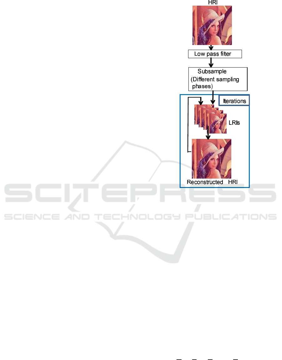
Figure 1 shows the basic idea of SRR (Farsiu et al.,

2004). The ﬁrst step is to process the HRI with a low

pass ﬁlter (LPF). The cut-off frequency of the LPF is

higher than the Nyquist frequency of the LRIs. LRIs

are created from HRI with sub-sampling and all LRIs

have aliasing. All LRIs are distinct since the sampled

pixel phases of each LRI are different. The summa-

Figure 1: SRR algorithm.

tion of sampled pixels exceeds the pixels in the HRI.

For example, suppose we want to make 256 256 pixel

LRIs from a 512 512 pixel HRI. In this case, four

LRIs would have the same pixels as the HRI; how-

ever, SRR must create more than four 256 256 images

to reconstruct HRI. That is, we need a larger amount

of information than is in the HRI in order to recon-

struct it with SRR. The LRIs are thus composed by

iteration, minimizing the cost function to recreate the

HRI.

There have been several SRR proposals for

the cost function (Farsiu et al., 2004)(Park et al.,

2003)(Panda et al., 2011)(van Eekeren et al., 2010).

They all have a similar aim to minimize the cost func-

tion, which comprises the sum of L

. In particular,

and L

are commonly used. L

is called the Norm

and n = 1, 2, ···. Minimizing the cost function (1) was

proposed by (Farsiu et al., 2004) , that of (2) was pro-

posed by (Panda et al., 2011) and that of (3) is pro-

posed by (van Eekeren et al., 2010).

= ||Y − HX||

+ λγ(X) (1)

J(X) = ||Y − HY||

+ λ||X||

(2)

SIGMAP 2017 - 14th International Conference on Signal Processing and Multimedia Applications

p, f

KMδ

∑

k=1

∑

m=1

k,m

− ey

k,m

(p, b, f))

(3)

h+v=1

∑

h,v=0,1

||f− S

f||

(

||P||

)

∑

p=1

(P)

It is not, however considered to be possible to de-

ﬁne just one cost function for all the various images.

Although one cost function may produce a good re-

sult for one image, it may give a poor result for an-

other image for which a different cost function gives

a better result (Farsiu et al., 2004).

However, it is not possible to dene one cost func-

tion for all the various images. Although one cost

function may produce a good result for one image, it

may give a poor result for another image (Farsiu et al.,

2004). The iterations are essential for SRR to recon-

struct HRI from LRIs. The result of iterations must

converge to the HRI. However, the result may diverge

if the cost function or some other functions such as

sampling phases are not appropriate. The number of

iterations is also an issue. The time consumed by the

iterations is in proportion to their number. A small

number is required for practical applications. Much

research has already gone into ﬁnding solutions to

these problems, which are called Fast and Robust. In

our opinion, much more important issues such as the

ultimate highest resolution produced with SRR need

to be addressed. If the convergence point of SRR is

just the HRI, as shown in Figure 1, SRR would not

improve the resolution of the original HRI at all.

The algorithm in Figure 1 shows that the role of

the LPF is very important. Without the LPF Figure 1,

the process is just breaking down the HRI into LRIs

and reconstructing the HRI with LRIs. It is just mak-

ing a jigsaw puzzle with the LRIs and then solving it

again by minimizing the complex cost function. The

result resolution of SRR depends on the characteris-

tics of the LPF and it is necessary for LRIs to contain

aliasing (Farsiu et al., 2004)(Glasner et al., 2009).

Figure 2: Example of LRI (taken from (Farsiu et al., 2004)).

The typical LRIs for SRR for a video are shown

in Figures 2 and 3 (Farsiu et al., 2004)(van Eekeren

et al., 2010). Images in Figures 2 and 3 are taken

Figure 3: Example of LRI (taken from (van Eekeren et al.,

2010)).

Figure 4: Moving object (Digital still camera).

Figure 5: Moving object (Video camera).

with an infrared camera. Infrared cameras have very

high sensitivity compared with general HDTV video

cameras and SDTV video cameras. Although these

images were taken by video cameras, there is not mo-

tion blur. It has not been mentioned that SRR can-

not work images that has motion blur. This is one

of the limitations of SRR. Digital still cameras can

take photographs at high shutter speeds. Some pro-

fessional video cameras shutters can reduce motion

blur. However, we rarely can use a shutter even if

the video camera has it because the photoelectric sen-

sors of video cameras do not have high sensitivities.

If we use the shutter in a professional video camera,

the resulting images may be very noisy Figures 4 and

5 are photographs taken of the same object with a

digital still camera and a video camera and are dis-

played at HDTV resolution. Since we are discussing

SRR for videos, cameras and displays must be com-

patible with HDTV resolution as a general standard

for video systems. There are other special cameras

such as high speed cameras and infrared cameras and

special displays such as Super HDTV (SHV) displays

and high dynamic range displays. However, they do

not fall into the general category. While Figure 4 has

details and aliasing around the moving object, Figure

5 does not have any. The difference between them

was caused by the shutter.

It is necessary for LRIs for SRR to have aliasing.

The block shapes in Figure 2 and Figure 3 are caused

by aliasing. In particular, when the image in Figure 3

was taken, the camera was gently shaken to provide

Performance of Blind Deconvolution and Super Resolution Image Reconstruction

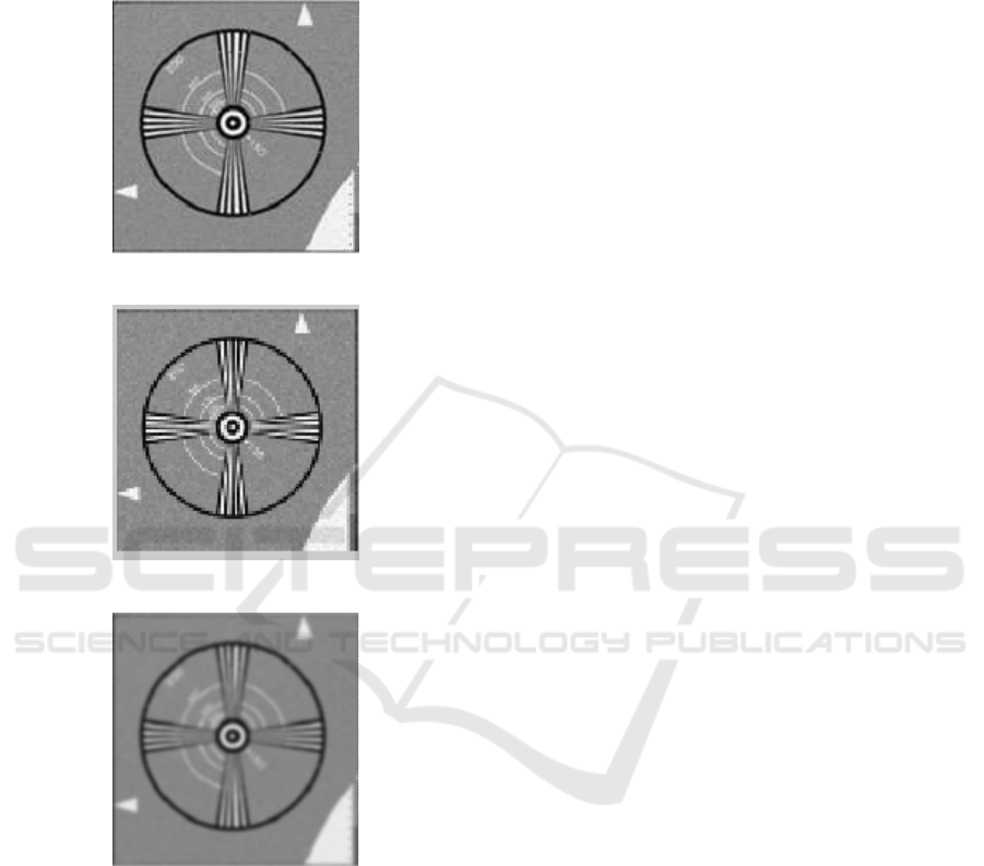
sub-pixel motion within the ﬁeld of view of the cam-

era (van Eekeren et al., 2010). This condition would

not occur in practical applications such as movie con-

tent and TV content.

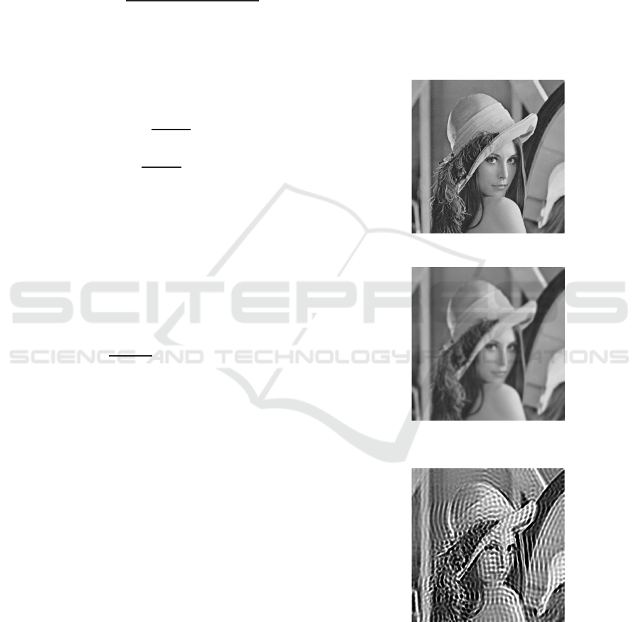
Figure 6: HRI.

Figure 7: LRI for SRR.

Figure 8: Blurry image.

3 MEANING OF SR

Here we have to think about the meaning of SR.

Whenever the term SR is used, it signiﬁes a way

of improving resolution. In an earlier SR research,

the original image was the HRI shown in Figure 6.

LRIs were made using the algorithm shown in Fig-

ure 1. HRI was processed with a low pass ﬁlter and

subsampled to create LRIs. Figure 7 shows an LRI

characteristic of those discussed in SRR papers. It

is over-sharpened with aliasing due to high frequency

elements. According to the Nyquist theorem, a pre-

ﬁlter is necessary to reduce the bandwidth not to cause

aliasing. In most cases, as far as the SR research goes,

LRIs are created under the conditions that do not meet

the requirements of the Nyquist sampling theorem.

It means making LRIs with aliasing and then recon-

structing the HRI from those LRIs by reducing alias-

ing. If the LRIs were created under the conditions of

the Nyquist sampling theorem, they would not have

the aliasing shown in Figure 8. If Figure 8 was used

as the LRI, SRR would not be able to reconstruct the

HRI.

We have to think about the meaning of SR and

LRI. For the practical application of the SR technique,

the image needs to be enlarged and the details of the

image need to be enhanced. Enlarging an image al-

ways causes enlargement blur. It does not create the

image shown in Figure 7 but the image shown in Fig-

ure 8. Figure 8 should be used as the input LRI for

SR to process and improve its resolution. Moreover,

many LRIs are not suitable for practical applications.

In general, we can use only one LRI. The conclusion

of this Section is that SR would improve resolution

from only one of the blurred images: the one shown

in Figure 8.

4 BLIND DECONVOLUTION (BD)

4.1 BD Algorithm

When we capture an image of an object, we capture

the beams of light that are reﬂected on the surface

of the object. After being reﬂected, the beams are

diffracted, diffused, and/or reﬂected in the space and

lens of the camera until they reach the imaging de-

vice in the camera. These factors degrade resolution

and make the images blurry. Here we deﬁne ψ(x, y)

as the true image and φ(x, y) as the observed blurry

image. (x, y) denotes the two dimensional vector. The

relationship between ψ(x, y) and φ(x, y) (Richardson,

1972a)(Lucy, 1974) can be presented as follows.

φ(x, y) =

Z Z

ψ(ξ, η)P(x− ξ, y − η)dξdη (4)

Here, ξ and η are introduced to calculate the horizon-

tal and vertical convolution.

ψ(x, y) =

Z Z

φ(ξ, η)Q(x− ξ, y− η)dξdη (5)

Here, P(·, ·) is the blur factor and Q(·, ·) is the

inverse ﬁlter of P(·, ·) (Richardson, 1972a). P(·, ·)

is called the point spread function (PSF) and gener-

ally it has a Gaussian shape characteristic (Richard-

son, 1972a). These are ﬁltering processes between

φ(x, y)and p(x, y).

SIGMAP 2017 - 14th International Conference on Signal Processing and Multimedia Applications

The blurry image can be restored by ﬁnding

P(x, y). Since this is a typical inverse problem, it is

impossible to solve it using a direct method (Petrou

and Edition, 2011). Instead, of a direct method, an

iterative method is proposed. Lucy, 1974 showed that

φ(x, y) can be obtained as follows. Using the Bayesian

inference, we obtain the following equation.

(x− ξ, y− η) =

(x− ξ, y− η)ψ

(x, y)

(6)

Here r is the iteration number. In Equation (5),

φ(ξ, η) is the original blurry image and we deﬁne it

as φ

(ξ, η) as the initial image.

Plugging Equation (6) into Equation (5), we ob-

tain the following formula.

r+1

(x, y) =

Z Z

(x, y)

(x− ξ, y− η)dξdη

= ψ

(x, y)

Z Z

(x, y)

(x− ξ, y− η)dξdη

(7)

Here, we transform Equation (4) with the iteration

number r.

(x, y) =

Z Z

(x− ξ, y− η)P

(ξ, η)dξdη (8)

Using Equation (6), we also obtain the recursion

equation of r about PSF,

r+1

(x, y)

= P

(x, y)

Z Z

(x, y)

(x− ξ, y− η)dξdη (9)

We deﬁne a scalar value E(r) to evaluate the con-

vergence.

E(r) =

Z Z

|φ

(x, y) − φ

r−1

(x, y)|dxdy (10)

Equation 10 is called L1 norm. Equation 10 is an in-

dicator of the iterations process. It decreases during

the convergence process.

Using the recursion Equations (7), (8), (9), Equa-

tion 10 and the iterations, we can obtain ψ(x, y), HRI

and P(x, y), PSF. The algorithm is called the Lucy

(Lucy, 1974) and Richardson (Richardson, 1972b) al-

gorithm and it is used in astronomy to refocus images

of planets star constellations.

4.2 Problems of BD

BD is a method for calculating the true image and PSF

together with iterations. During the iterations, the

blurry image and PSF gradually converge to the true

image and the true PSF. However, the iterations some-

times causes divergences or fall down to the limit cy-

cles. In these cases, the BD cannot create the true

image and PSF. Figure 9 is the original image. Figure

10 shows a blurry image that is created from Figure 9

processed with a Gaussian low pass ﬁlter (σ = 3.0,

kernel 15 × 15). If we use BD for Figure 10, BD

causes divergence that creates Figure 11 as the result

image and Figure 12 as PSF. In the BD process the

shape of PSF is very important. Figure 13 shows a

typical shape of PSF. However, the PSF shape of Fig-

ure 12 spreads in diagonal directions that emphasize

oblique frequency elements. The oblique frequency

elements amplify oblique edges and create the diago-

nal ringing shown in Figure 11. It is a kind of diver-

gence.

Figure 9: Original image.

Figure 10: Gaussian ﬁlter (σ = 3.0 kernel 15 ×

15)processed.

Figure 11: Example of divergent image.

4.3 Proposed Method

In general, our interests tend to focus on the quality

of the resulting image. However, in the BD process,

image degradation is caused by the irregular shape of

Performance of Blind Deconvolution and Super Resolution Image Reconstruction

Figure 12: Example of divergent PSF.

Figure 13: Example of PSF.

PSD. We investigated the change of the PSD shape

during the iterations and made an interesting observa-

tion. In the BD iteration process of the previous sec-

tion, Figure 10, the PSF became Figure 14. Although

in general, PSD has symmetrical Gaussian shape, Fig-

ure 14 is asymmetrical. The asymmetrical PSF gen-

erates a divergent image during the iterations. When

the E(r) value of Equation 10 increases, we rotate the

PSF form 180

, arriving at Figure 15, and then con-

tinue the iterations. This process produced the PSF

shown in Figure 16 and the resulting image is shown

in Figure 17. Compared with Figure 10, Figure 17 has

been restored and it has higher resolution. According

to the experiments, the rotation introduced into the

PSF method works when the iterations causes diver-

gence. According to our simulations, it also decreases

limit cycles.

Figure 14: Asymmetry PSF.

Figure 15: Rotation PSF of Figure 14.

Figure 16: Convergence PSF of Figure 14.

Figure 17: BD processed image for 10.

5 EXPERIMENT

Since SRR is one of the most common SR techniques,

we compare the performance of BD with that of SRR.

The algorithm of SRR that creates HR from LRIs is

explained in Section 2 and Figure 1. Instead of SRR,

we use BD to improve the resolution of an image,

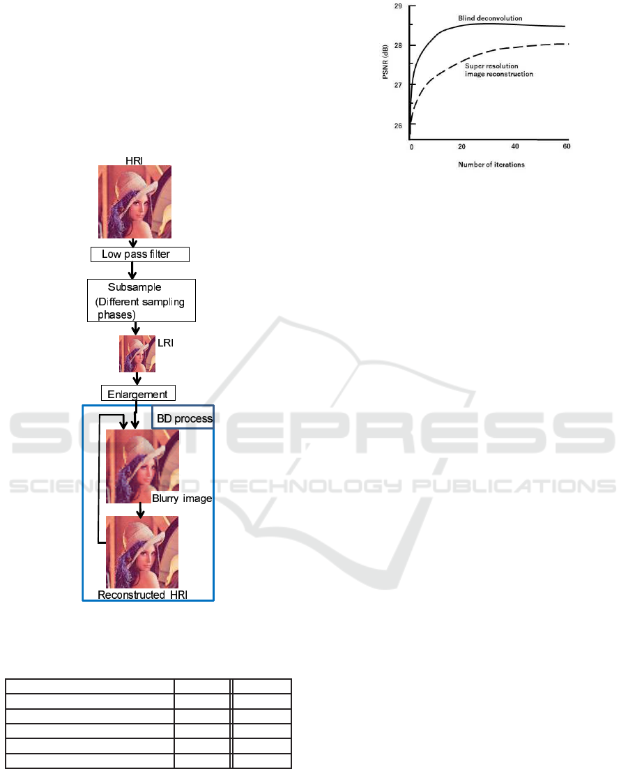
as shown in Figure 18. HRI is processed with a low

pass ﬁlter (LPF) to limit the bandwidth and subsam-

ple to create a LRI. LRI is enlarged with a digital ﬁlter

and a blurry image is obtained. The blurry image is

processed with BD and HRI is created. Both SRR

and BD can create HRI from LRIs/LRI. Two points

should, however, be noted. First, SRR needs multi-

ple LRIs, whereas BD needs only one LRI. Second,

the characteristics of LPFs are different. In SRR (Fig-

ure 1), the bandwidth of the LPF is wide and alias-

ing occurs when LRIs are created. In contrast, in the

LPF in Figure 18, the LRI created by the subsam-

ple does not have aliasing. Therefore, the bandwidth

of LPF is narrow enough to satisfy the Nyquist sam-

pling theorem. In SR, the quality of the reconstructed

HRI is the most important. Many SRR papers evalu-

ated qualitatively the outputs from their applications

of SRR, i.e., the comparison between the original HRI

and the reconstructed HRI in Figure 18. Here we eval-

uate SRR and BD quantitatively with the peak signal

to noise ratio (PSNR). Although there are many SRR

papers, most of them include only a qualitative com-

parison. We chose four papers that show the PSNR

values (Youmin et al., 2016) (Yin et al., 2016) (Shah

et al., 2013) (Jahanbin and Naething, 2005). Their

subsample ratios are 2:1, i.e., the same as the algo-

rithm shown in Figure 18. We conducted computer

simulations of the proposed BD algorithm. The im-

ages used are the famous ones of Lena and Mandrill.

In our simulations, the resolution of HRI is 512× 512

and that of LRI is 256 × 256, which means the sub-

sample ratio is 2:1. Table 1 shows the comparison re-

sults between the proposed BD method and SRR. In

two papers (Youmin et al., 2016) (Shah et al., 2013),

SIGMAP 2017 - 14th International Conference on Signal Processing and Multimedia Applications

Mandrill was not used. Table 1 shows that the perfor-

mance of BD as the SR capability outperforms SRR.

Initially, BD was proposed for astrophotography

to improve the out-of-focus images. However, we

have shown in this paper that BD can be used for

SR and outperform the most common SR techniques.

Due to space limitations, the comparison between

learning-based SR and BD cannot be discussed here.

This is the next step in this research.

Figure 18: BD algorithm.

Table 1: Quantitative Performance Comparison Using

PSNR.

Lena Mandrill

(Youmin et al., 2016) 29.2142 -

(Yin et al., 2016) 23.4060 22.2895

(Shah et al., 2013) 23.3731 -

(Jahanbin and Naething, 2005) 23.509 19.461

Proposed method 35.041d 24.164

Figure 19: Convergence speed of BD and SRR.

6 SPEED OF CONVERGENCE

BD and SRR need iterations to converse on the HRIs.

Figure 19 shows the relations of the BD and SRR. The

horizontal axis is the iteration number and the verti-

cal axis is the peak signal to noise ratio (PSNR). The

two curves show the changes of PSNR to the itera-

tions. As the iteration progresses the PSNR values

improve. However, the behaviors of the PSNR values

of BD and SRR are different. The PSNR value of BD

is better than that of SRR and it is almost saturated at

the 20 times iterations. It means that BD converges

on HRI faster than SRR. Iterations are heavy load for

SR technologies. If the numbers of the iterations be-

come smaller, it means the decreasing of the calcula-

tions costs. According to the simulation result, BD is

superior to SRR about the cost.

7 CONCLUSION

The capability of BD is discussed. BD was pro-

posed to refocus astrophotographs. This is a similar

idea to SR, which creates HRI from LRIs. However,

BD comes with some issues, such as falling in diver-

gences or limit cycles. In this study, a method to ﬁx

these issues was proposed. Using this method, BD ca-

pability was compared with the typical SR technique,

SRR. According to the simulation results, BD outper-

formed SRR about the image quality and cost. Com-

paring BD with another common SR, learning-based

SR is the next step.

REFERENCES

Andrews, H. and Hunt, B. (1997). Digital Image Restora-

tion. Englewood Cliffs, N.J. : Prentice-Hall.

Banha, M. and Katsaggelos, A. (1997). Digital image

restoration.

Performance of Blind Deconvolution and Super Resolution Image Reconstruction

IEEE Signal Processing Magazine, 14(2):24–41.

Bannore, V. (2009). Iterative-Interpolation Super-

Resolution Reconstruction. Springer.

Begin, I. and Ferrie, F. R. (2004). Blind super-resolution

using a learning-based approach. ICPR 2004, 2:85–

89.

Chaudhuri, S. (2001). Super-Resolution Imaging. Kuliwer

Academic Publishers.

Chaudhuri, S. and Manjunath, J. (2005). Motion-Free

Super-Resolution. Springer.

Devi, A. G., Madhu, T., and Kishore, K. L. (2014). An

improved super resolution image reconstruction us-

ing svd based fusion and blind deconvolution tech-

niques. International Journal of Signal Processing,

Image Processing and Pattern Recognition.

Elad, M. and Feuer, A. (1997). Restoration of a single su-

perresolution image@from several blurred, noisy, and

undersampled measured images. IEEE Trans. Image

Processing, 6(12):1646–1658.

Farsiu, S., Robinson, D., Elad, M., and Milanfar, P. (2004).

Fast and robust multi-frame super-resolution. IEEE

Transactions on Image Processing.

Glasner, D., Bagon, S., and Irani, M. (2009). Super-

resolution from a single image. International Con-

ference on Computer Vision (ICCV).

Harmeling, S., M. Hirsch, S. S., and Scholkopf, B. (2009).

Online blind image deconvolution for astronomy.

IEEE Conference on Comp. Photogr.

Harmeling, S., Sra, S., Hirsch, M., and Scholkopf, B.

(2010). Multiframe blind deconvolution, super-

resolution, and saturation correction via incremental

em. Proceedings of 2010 IEEE 17th International

Conference on Image Processing, pages 3313–3316.

Jahanbin, S. and Naething, R. (2005). Super-resolution im-

age reconstruction performance.

Katsaggelos, A., Molona, R., and Mateos, J. (2007). Super

Resolution of Images and Video, Synthesis Lectures on

Images, Video and Multimedia Processing. Morgan &

Clayppo Publishers.

Lucy, L. B. (1974). An iterative technique for the recti-

ﬁcation of observed distributions. The Astronomical

Journal, 79(6):745–754.

Panda, S., Prasad, R., and Jena, G. (2011). Pocs based

super-resolution image reconstruction using an adap-

tive regularization parameter. IEEE Transactions on

Image Processing.

Park, S. C., Park, M. K., and Kang, M. G. (2003).

Super-resolution image reconstruction: A technical

overview. IEEE Signal Processing Magazine.

Patti, A. and Altunbasak, Y. (2001). Artifact reduction

for set theoretic super resolution image reconstruction

with edge adaptive constraints and higher-order inter-

polants. IEEE Trans. Image Processing, 10(1):179–

186.

Patti, A., Sezan, M., and Tekalp, A. (1997). Superresolution

video reconstruction@with arbitrary sampling lattices

and nonzero aperture time. IEEE Trans. Image Pro-

cessing, 6(8):1064–1076.

Petrou, M. and Edition, C. P. S. (2011). Image Processing:

the Fundamentals. WILEY, United Kingdom.

Pratt, W. K. (2001). Digital Image Processing (3rd Ed):

New York. John Wiley and Sons.

Protter, M., Elad, M., Takeda, H., and Milanfar, P. (2009).

Generalizing the nonlocal-means to super-resolution

reconstruction. IEEE Transactions on Image Process-

ing.

Richardson, W. H. (1972a). Bayesian-based iterative

method of image restoration. Journal of the Optical

Society of America, 62(1).

Richardson, W. H. (1972b). Bayesian-based iterative

method of image restoration. Journal of The Optical

Society of America, 62(1):55–59.

Sanchez-Beato, A. and Pajares, G. (2008). Nonitera-

tive interpolation-based super-resolution minimizing

aliasing in the reconstructed image. IEEE Transac-

tions on Image Processing, 17(10):1817–1826.

Schreiber, W. F. (1970). Wirephoto quality improvement by

unsharp masking. J. Pattern Recognition, 2:111-121.

Shah, K., Pandya, J., and Vahora, S. (2013). A survey on

super resolution image reconstruction techniques. In-

ternational Journal of Engineering Research & Tech-

nology (IJERT), 2(4):1897–1901.

Sroubek, F., Cristobal, G., and Flusser, J. (2007). A uniﬁed

approach to superresolution and multichannel blind

deconvolution. IEEE Transactions on Image Process-

ing, 16(9):2322–2332.

van Eekeren, A. W. M., Schutte, K., and van Vliet, L. J.

(2010). Multiframe super-resolution reconstruction of

small moving objects. IEEE Transactions on Image

Processing.

Yin, Y., Ruan, Q., and Zhang, T. (2016). An improved

super-resolution image reconstruction algorithm. In-

ternational Journal of Signal Processing, Image Pro-

cessing and Pattern Recognition, 9(3):103–112.

Youmin, G., Xing, Z., Yanning, G., and Zhen, D. (2016).

An experimental comparison of super-resolution re-

construction for image sequences. Proceedings of the

35th Chinese Control Conference.

SIGMAP 2017 - 14th International Conference on Signal Processing and Multimedia Applications