
Autonomous Trail Following
Masoud Hoveidar-Sefid and Michael Jenkin
Electrical Engineering and Computer Science Department and York Centre for Field Robotics,
Lassonde School of Engineering, York University, Toronto, Canada
Keywords:
Autonomous Navigation, Trail Following, Path Finding.
Abstract:
Following off-road trails is somewhat more complex than following man-made roads. Trails are unstructured
and typically lack standard markers that characterize roadways. Nevertheless, trails can provide an effective
set of pathways for off-road navigation. Here we approach the problem of trail following by identifying trail-
like regions; that is regions that are locally planar, contiguous with the robot’s current plane and which appear
similar to the region in front of the robot. A multi-dimensional representation of the trail ahead is obtained by
fusing information from an omnidirectional camera and a 3D LIDAR. A k-means clustering approach is taken
based on this multi-dimensional signal to identify and follow off-road trails. This information is then used to
compute appropriate steering commands for vehicle motion. Results are presented for over 1500 frames of
video and laser scans of trails.
1 INTRODUCTION
Trail following is a hard problem in comparison with
the well known autonomous road following which is
aided by many detectable and well known features
available in highways and streets. As is the case for
the road following algorithm, the goal of the trail fol-
lowing algorithm is to process sensor data so as to
produce motion commands that drive the robot along
the trail and centre the robot on it. Any trail follow-
ing algorithm is informed by the data of the sensors
that are connected to the robot. More sensors pro-
vide an advantage for more robust sensing and hence
a more robust algorithm. The work presented here
relies on the fusion of vision and LIDAR informa-
tion and then segmenting the fused datasets using a k-
means clustering algorithm into ‘trail’ and ‘non-trail’
regions based on the assumption that the robot is cur-
rently on the trail, and that the region directly in front
of the robot is “trail-like”. Based on this clustering
process, a motion command is constructed to drive
the robot along the trail and to centre the robot on it.
2 PREVIOUS WORK
There is a large road following literature associated
both with ‘off-road’ roads as well as hard surface
roadway following. Previous work on path finding
and following task can be classified based on the sen-
sors employed in three different categories: visual ap-
proaches, laser approaches and integrated vision-laser
approaches.
Vision-based Approaches: Vision-based follow-
ing approaches can be traced back to the 1980’s
(e.g., (Waxman et al., 1985),(Kuan et al., 1988) and
(Liou and Jain, 1987)), and research in this field
continues to today. It is not practical to review
all approaches here (see (DeSouza and Kak, 2002),
(Bar Hillel et al., 2014) and (Buehler et al., 2007)
for reviews), but rather a few examples are used to
illustrate the vast number of different approaches.
(Moghadam et al., 2010), present a self-supervised
learning algorithm for terrain classification that ex-
ploits near-field stereo vision in front of the robot
and combines this information with terrain features
extracted from monocular vision. (Moghadam and
Dong, 2012) use an alternative approach for road di-
rection estimation, based on the vanishing point of the
road. The algorithm first localizes the vanishing point
based on one image frame and then uses a sequence
of images to predict the direction of the given road.
Laser-based Approaches: The main advantages of
using a LIDAR sensor are that they provide a 3D rep-
resentation of the environment and operate indepen-
dently of the lighting conditions. The major disad-
vantages of LIDAR sensors are their lack of dense
resolution and their need to emit energy into the en-
viornment. Many LIDAR sensors are able to return
Hoveidar-Sefid, M. and Jenkin, M.
Autonomous Trail Following.
DOI: 10.5220/0006468404250430
In Proceedings of the 14th International Conference on Informatics in Control, Automation and Robotics (ICINCO 2017) - Volume 2, pages 425-430
ISBN: Not Available
Copyright © 2017 by SCITEPRESS – Science and Technology Publications, Lda. All rights reserved
425

the intensity of the points as well which can be ex-
ploited when detecting different suface features inde-
pendently from the lightning (see (von Reyher et al.,
2005), (Kammel and Pitzer, 2008) and (Ogawa and
Takagi, 2006)). As an example, (Kammel and Pitzer,
2008) used LIDAR intensity values to detect the lane
markings due to their cue difference from the back-
ground (i.e., road) and to extract the curb’s position
on the road based on the height change in the laser
range finder data. (Hern
´
andez and Marcotegui, 2009)
and (Cremean and Murray, 2006) used LIDAR to de-
tect the curbes and consequently the edges of the road
ahead. Single beam LIDAR sensors are only able to
detect obstacles and features in the plane of the laser
beam. Multiple 2D LIDAR sensors or 3D laser scan-
ners, detect more features of the environment. An
improved road detection and following scheme (see
(Kammel and Pitzer, 2008) and (Thrun et al., 2006),
for example) can be achieved using multiple LIDAR
scanners in comparison to the single 2D LIDAR ap-
proach (see (von Reyher et al., 2005) and (Zhang,
2010), for example).
Integrated Vision-laser-based Approaches: The in-
tegration of more sensors can enhance environmental
perception. Fusing both visual information and laser
range information enables a robot to have a more ro-
bust perception of the surrounding environment and
the trail within it. (Rasmussen, 2002) describes an
approach with a laser range finder and camera for
the road following task, using four different features;
height and smoothness of the points in front of the
robot and color and texture features obtained from
an on-board camera. Rasmussen used a neural net-
work to classify different kinds of roads (paved or
unpaved) using data sets of images and laser infor-
mation from similar road scenarios. In the DARPA
Grand Challenge in 2005 (DARPA, 2016), the Stan-
ley robot, which won the competition, used a combi-
nation of vision and laser range finder for task of road
detection in off-roads and desert terrains (Thrun et al.,
2006). Equipped with five 2D laser range finders,
Stanley was able to classify the terrain to three differ-
ent classes; obstacle, drivable and unknown. An ob-
stacle is defined on a grid cell around the robot which
two nearby points of data have a height difference of
more than a defined vertical distance threshold. Using
this map of the road, Stanley computed a quadrilat-
eral in front of the robot containing all possible driv-
able grid cells and used this region to perform color
classification of the further road ahead to increase the
range of road detection. Stanley could maintain high
speeds in navigation and was able to handle the sud-
den changes in the surface type of the road as well.
Although there have been considerable successes
(a) (b)
Figure 1: Coordinate frames. (a) shows the robot coordinate
frame placed underneath the center of mass of the robot on
the ground plane at point p = (x,y, z). (b) shows a bird’s
eye view of the robot on the path in two subsequent frames
at time t and t + ∆t with its position and orientation in the
world coordinate frame.
in the navigation of roadways by autonomous sys-
tems, such algorithms are not necessarily well suited
for trail following as trails typically lack the formal
structure of roadways. Here we consider the problem
of following trails which are characterized by provid-
ing a continuous ground plane upon which to travel
and a visual and structure appearance that is differ-
ent from the surrounding environment and consistent
with the view in front of the robot.
3 PROBLEM DEFINITION
For trail following, it is assumed that the robot is on
the trail at time t, and the goal is to obtain the local
twist vector (V,ω) that moves the robot along the trail
while centering the robot on it. so that the robot has
moved along the trail and is (more) centered on it at
time t+1. Specifically, it is assumed that
• The robot is on the trail (p
t
is on trail).
• The robot is more or less centered on the trail and
looking along the trail.
• The path on the trail is more or less flat (i.e., the
trail is drivable by the robot).
• The trail is characterized by sensor features which
differentiate it from the surroundings.
The robot combines visual and range informa-
tion from the local environment and labels the region
around the robot as either trail or non-trail based on
the assumptions above. The goal of the algorithm is
to (i) detect that there exists a drivable trail in front of
the robot (the assumptions above are met), and if so
(ii) to characterize the trail and to estimate the twist
vector that will cause the robot to move forward along
the trail and center itself on it (see Fig. 1).
ICINCO 2017 - 14th International Conference on Informatics in Control, Automation and Robotics
426

4 TRAIL FOLLOWING
The basic approach followed here is to construct a
hyper-dimensional image that characterizes both de-
viation from the ground plane and per pixel image
information, and then assuming that the robot is cur-
rently on the trail to utilize the k-means clustering al-
gorithm on a reduced dimensional version of this im-
age to identify trail versus non-trail locations. This
information is then used to construct a local mo-
tion command (twist vector) that will drive the robot
along the trail and keep the robot centered on it. An
overview of the approach is shown in Fig. 2.
The algorithm utilizes both wide field visual and
LIDAR data. Data is obtained from a Velodyne HDL-
32E 3D laser scanner (velodyne, 2016) that obtains
a 360 degree view of the space and a forward-facing
Kodak Pixpro SP360 camera (kodak, 2016) mounted
on the front of the robot.
4.1 Processing The Laser Data
Many methods have been used to extract different fea-
tures of point cloud datasets. Prior knowledge about
the characteristic of the plane can help in extracting a
more accurate plane model. Robust algorithms such
as RANdom SAmpling Consensus (RANSAC) (Fis-
chler and Bolles, 1981) and M-estimator SAmpling
Consesus (MSAC) (Torr and Zisserman, 2000) have
been used successfully to extract plane information
from laser data. Here we exploit the fact that we are
interested in grouping data points that correspond to
the ground plane that is currently supporting the ve-
hicle. That is, planes that pass near p = (0,0,0) and
that have a normal near ˆn = (0,0,1). A simplified
version of the MSAC plane fitting algorithm (Algo-
rithm 1) is used to find the plane that best fits the laser
dataset while grouping laser points into inlier and out-
lier groups. Triplets of points (p
1
, p
2
, p
3
) are repeat-
edly extracted from the point cloud and used to form
a plane that is consistent with ˆn = (0,0,1). Then each
point in the dataset is tested against this plane. Points
are identified as either inliers or outliers based on the
distance from the point to the plane. A cost fit func-
tion is computed as the sum of the distances from the
plane for inliers plus the cutoff distance for outliers.
This score function is then used to select the ‘best fit’
plane and to identify the inlier/outlier sets. As shown
in Fig. 2, laser data is first clipped to the region in
front of the robot. The resulting data is then used
within the MSAC plane fitting algorithm to determine
a cost function that represents the deviation from the
robot ground plane for each laser reading. This cost
function is then mapped into the camera image and
the two signals integrated.
Algorithm 1: M-estimator SAmpling Consensus algo-
rithm (Torr and Zisserman, 2000) for plane fitting.
1: Input (P[x,y, z], θ
th
, ˆn
P
,N
trials
,δ)
2: for a = 1 : N
trials
do
3: for non-colinear random points p
1
, p
2
, p
3
∈
P[x,y, z] do
4: if cos
−1
( ˆn
S
a
· ˆn
P
) < θ
th
then
5: remove p
1
, p
2
, p
3
from P[x,y, z]
6: for all [x
i
,y
i
,z
i
] ∈ P[x, y,z] do
7: e
i
= |distance(S
a
,[x
i
,y
i
,z
i
])|
8: if e
i
≤ δ then
9: ρ(e
i
) = e
i
10: add {[x
i
,y
i
,z
i
]} to P
inliers
a
11: else
12: ρ(e
i
) = δ
13: add {[x
i
,y
i
,z
i
]} to P
outliers
a
14: C
a
=
∑
i
ρ(e
i
)
15: k = argmin
j
{C
j
}
16: return C
k
, P
inliers
k
, P
outliers
k
4.2 Processing the Visual Data
In order to integrate the visual data with the data from
the LIDAR, the camera must be calibrated. A mathe-
matical model of omnidirectional cameras and a cali-
bration method using a planar checkerboard target are
described in (Micusik and Pajdla, 2003) and (Scara-
muzza et al., 2006) respectively. Let X
i
be a 3D point
in world coordinates. Then let u
00
= [u
00
,v
00
]
T
be the
projection of X
i
on the sensor plane and u
0
= [u
0
,v
0
]
T
is the projection of point u
00
on camera plane. u
0
and
u
00
are related to each other by an affine transforma-
tion due to miss-alignment of the camera and sen-
sor plane axes and digitizing process of light rays to
pixels. u
00
can be described as u
00
= Au
0
+ t, where
A ∈ ℜ
2×2
and t ∈ ℜ
2×1
. Define a projection func-
tion g, relating a u
00
point on the sensor plane to a
vector pointing out of the camera origin O to the cor-
responding 3D point X
i
. The resulting camera model
is given by λ.g(u
00
) = λ.g(Au
0
+t) = PX
i
, λ > 0. This
treats X
i
∈ ℜ
4
as a homogeneous point [x,y, z, 1]
T
,
P ∈ ℜ
3×4
as a perspective transformation matrix and
λ is the normalized distance to X
i
. In order to cali-
brate the camera, A and t matrices and the function
g should be estimated. Using this estimation we can
extract a vector pointing to the scene point from point
O to every point X
i
. g is a non-linear function and
is defined as g(u
00
,v
00
) = (u
00
,v
00
, f (u
00
,v
00
))
T
, where
f is a rotationally symmetric function with respect
to the axis of the sensor. Function f is modeled as
f (u
00
,v
00
) = a
0
+ a
1
ρ + a
2
ρ
2
+ ... + a
n
ρ
n
, where the
model parameters are a
i
, i = 0,1,2,...,n and n is the
degree of the polynomial. ρ is the Euclidean dis-
Autonomous Trail Following
427
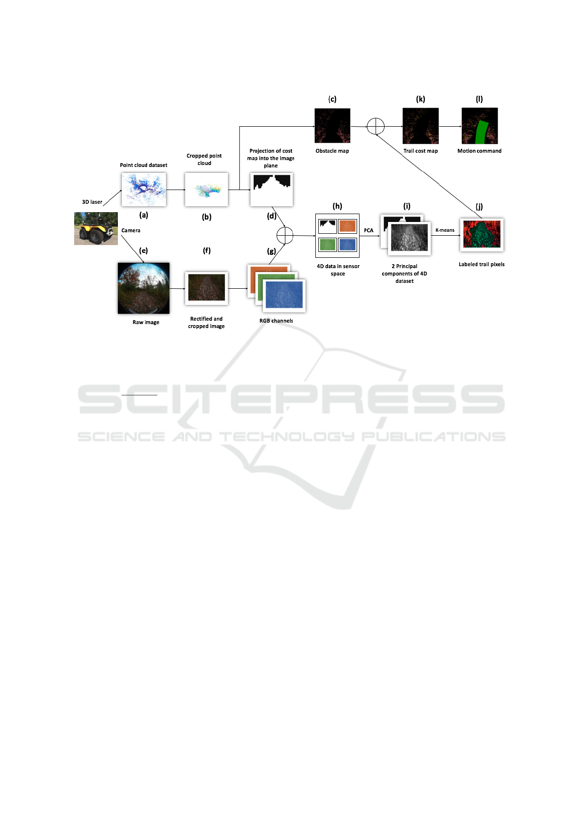
Figure 2: Data from the two sesnors are processed into a common reference frame. Laser data is recoded as error relative to
the expected ground plane. When integrated with the camera signal this produces a 4D sensor signal (r,g,b,e) which then goes
through a PCA process to obtain a 2D signal for segmentation. The k-means clustering algorithm is used to segment regions
similar to the region directly in front of the robot (which is assumed to be trail) from other regions.
tance of point (u
00
,v
00
) from sensor’s geometric center,
hence ρ =
√
u
002
+ v
002
. The completed approach to es-
timate these parameters is presented in more details in
(Scaramuzza et al., 2006). Calibration parameters are
used to define the relation between any 3D point in the
world coordinate and the pixel on the image plane.
4.3 Merging Vision and Laser
In order to integrate the data of camera and laser into
a single measurement vector, a common reference
frame is required. When integrated with the output of
the vision sensor this obtains a 4DOF signal (r,g,b,e)
where e is the remapped C
k
cost from the best plane
fitting function obtained from the laser data.
There is not necessarily a correspondence point
in point cloud dataset for every pixel in the image;
for this reason it is necessary to assign each obstacle
point P[x
i
,y
i
,z
i
] to a group of pixels
(u
c
,v
c
)
G instead,
where (u
c
,v
c
) is the position of the correspondence
pixel of the reprojection of point X
i
[x
i
,y
i
,z
i
] on the
image plane. This pixel group is created by dilating
the pixel (u
c
,v
c
).
Recognizing the redundant nature of this 4D sig-
nal and the cost associated with performing clustering
on high dimensional data, the dataset is then com-
pressed using principal component analysis (PCA)
[Abdi and Williams, 2010]. This allows the 4DOF
signal to be represented with a lower dimensional sig-
nal thus reducing the cost of the clustering algorithm.
4.4 Trail Following
In order to label pixels of an image to different groups,
k-means clustering (MacQueen et al., 1967) is used.
After applying this algorithm, the dataset is divided
into a defined number of clusters, where each clus-
ter is represented with a centroid and indexes of each
data entry belonging to that cluster. The k-means
clustering algorithm with a fixed number of k clus-
ters and a d dimensional dataset with n number of
entities can be solved in the order of O(n
dk+1
) (see
(Inaba et al., 1994)). After identifying the k clusters,
each cluster is represented by its mean µ
k
and covari-
ance matrix Σ
k
and is assigned to one of the two cat-
egories: trail, or non-trail. An immediate region in
front of the robot is assumed to contain all the char-
acteristics of the drivable trail. This region is called
Region of Interest on the Trail or ROIT. ROIT is se-
lected as a rectangle in the camera reference frame
and is modeled using a Mixture of Gaussian (MOG)
distributions. Pixels of ROIT are defined as g num-
ber of Gaussians with mean of µ
i
and covariance of
Σ
i
;{i = 1,2...,g}. Cluster k is counted as trail if it
similar to one of the g Gaussians in ROIT. This simi-
larity is determined through the Mahalanobis distance
as d(i, j) = (µ
i
−µ
j
)
T
(Σ
i
+Σ
j
)
−1
(µ
i
−µ
j
) where {i =
ICINCO 2017 - 14th International Conference on Informatics in Control, Automation and Robotics
428

(a) (b) (c) (d) (e) (f)
Figure 3: Results of the trail following algorithm on different sample trails. The point cloud data, obstacle mask in the image plane along
with the trail image, segmented mask of the drivable and non-drivable path on the trail with a green and red visualization of the outputs and
the predicted trajectory of the robot after the computed motion command are depicted sequentially for every frame. (a, b) show two frames
from the concrete dataset, (c, d) are two selected frames from the dirt trail and (e, f) show the results for the algorithm on an asphalt trail.
1,2...,g}and {j = 1,2...,k}. µ and Σ are the mean and
covariance matrices of each Gaussian distribution, re-
spectively. d(i, j) denotes the Mahalanobis distance
between the two distributions. For every cluster, if
d(i, j) is less than a threshold, the cluster is consid-
ered to be similar and it is labeled as trail, otherwise
it is identified as being different and the cluster repre-
sents a non-trail region. The results of this assignment
is shown in Fig. 2(j).
To update the 2D cost map (obtained with point
clouds) shown in Fig. 2(c) with the results of the clus-
tering algorithm (shown in Fig. 2(j)), each grid cell in
the 2D cost map that is assumed to be free space is
checked against the label of its corresponding pixel.
If the corresponding pixel of a grid cell labeled as
non-road, then the cost will be updated to the value
of
c
max
+c
min
2
, where c
max
is the highest cost (denoting
the existence of an obstacle) and c
min
represent a free
space.
Different rotational velocities coupled with a com-
mon forward motion velocity are considered, and the
trajectory with the minimum cost over a small tempo-
ral window is chosen.
5 EXPERIMENTAL RESULTS
Three different datasets have been recorded using the
on-board Kodak Pixpro SP360 camera and a Velo-
dyne HDL- 32E 3D laser scanner from the trails of
the campus of York University. These datasets were
captured on three different trail types: 1) a concrete
trail surrounded by grass and trees, 2) a dirt trail cov-
ered with leaves and 3) a pedestrian asphalt trail sur-
rounded with grass. Results of the algorithm on three
trail types are shown in Fig. 3.
In order to asses the accuracy of the trail following
algorithm, a set of 1500 natural images from the three
datasets were used. These images were hand labeled
by two human observers who were asked to label the
drivable path in each frame and these labeled images
were used as ground truth. A binary mask of these
labeled images is used to evaluate the accuracy of the
output of the algorithm. The labeled output of the al-
gorithm is also extracted as a binary mask. Using a
pixel-wise XNOR function on the ground truth mask
and output of the algorithm, by dividing the number
of pixels with the value of 1 (N
XNOR-pixels
) to the total
number of the pixels in the image (N
all-pixels
), accu-
racy of the algorithm on each frame is calculated as
(N
XNOR-pixels
/N
all-pixels
) ×100%.
Fig. 4 shows histograms of the calculated for each
of the three trail types. The overall accuracy of the
algorithm on the dirt dataset, asphalt dataset and con-
crete dataset is 60.85%, 86.3% and 96.8% respec-
tively.
6 CONCLUSION
In this paper we presented an adaptive trail follow-
ing algorithm for autonomous robot navigation on dif-
ferent types of trails, using visual information of the
environment, point cloud data obtained from the on-
board sensors. Finally, the output of the algorithm
on a diverse set of trail types were presented with
successfully detected trail and non-trail regions along
with a motion command to move the robot forward in
the environment.
ACKNOWLEDGMENTS
The support of NSERC Canada and the NSERC
Canadian Field Robotics Network (NCFRN) are
gratefully acknowledged. We would also like to thank
Autonomous Trail Following
429

(a) Concrete (b) Dirt (c) Asphalt
Figure 4: The accumulative accuracy histogram charts along side their corresponding frame with highest accuracy and its
hand labeled ground truth mask of (a) concrete, (b) dirt and (c) asphalt datasets respectively. These histograms show the
distribution of the frames based on their computed accuracy in comparison to the ground truth dataset.
Emmanuel Mati-Amorim and Arjun Kaura who hand
labeled the test datasets.
REFERENCES
Bar Hillel, A., Lerner, R., Levi, D., and Raz, G. (2014).
Recent progress in road and lane detection: a survey.
Machine Vision and Applications, pages 1–19.
Buehler, M., Iagnemma, K., and Singh, S. (2007). The 2005
DARPA Grand Challenge: The Great Robot Race,
volume 36. Springer Science & Business Media.
Cremean, L. B. and Murray, R. M. (2006). Model-based es-
timation of off-highway road geometry using single-
axis ladar and inertial sensing. In Proc. ICRA 2006.,
pages 1661–1666.
DARPA (2016). The Defense Advanced Research Projects
Agency (DARPA) website.
DeSouza, G. N. and Kak, A. C. (2002). Vision for mobile
robot navigation: A survey. IEEE PAMI, 24(2):237–
267.
Fischler, M. A. and Bolles, R. C. (1981). Random sample
consensus: a paradigm for model fitting with appli-
cations to image analysis and automated cartography.
Comm. ACM, 24(6):381–395.
Hern
´
andez, J. and Marcotegui, B. (2009). Filtering of ar-
tifacts and pavement segmentation from mobile lidar
data. In ISPRS Workshop Laserscanning 2009.
Inaba, M., Katoh, N., and Imai, H. (1994). Applications
of weighted voronoi diagrams and randomization to
variance-based k-clustering. In Proc. 10th Ann. Symp.
Comp. Geom., pages 332–339.
Kammel, S. and Pitzer, B. (2008). Lidar-based lane marker
detection and mapping. In 2008 IEEE Intell. Vehic.
Symp., pages 1137–1142.
kodak (2016). The Kodak camera website.
Kuan, D., Phipps, G., and Hsueh, A. C. (1988). Au-
tonomous robotic vehicle road following. IEEE PAMI,
10(5):648–658.
Liou, S.-P. and Jain, R. C. (1987). Road following using
vanishing points. Computer Vision, Graphics, and Im-
age Processing, 39(1):116–130.
MacQueen, J. et al. (1967). Some methods for classification
and analysis of multivariate observations. In Proc. 5th
Berkeley Symp. on Math. Stats. and Prob., volume 1,
pages 281–297. Oakland, CA, USA.
Micusik, B. and Pajdla, T. (2003). Estimation of omnidirec-
tional camera model from epipolar geometry. In IEEE
CVPR, volume 1, pages I–485.
Moghadam, P. and Dong, J. F. (2012). Road direction detec-
tion based on vanishing-point tracking. In IEEE/RSJ
IROS, pages 1553–1560.
Moghadam, P., Wijesoma, W. S., and Moratuwage, M.
(2010). Towards a fully-autonomous vision-based ve-
hicle navigation system in outdoor environments. In
ICARCV, pages 597–602.
Ogawa, T. and Takagi, K. (2006). Lane recognition us-
ing on-vehicle lidar. In IEEE Int. Vehic. Symp., pages
540–545.
Rasmussen, C. (2002). Combining laser range, color, and
texture cues for autonomous road following. In IEEE
ICRA, volume 4, pages 4320–4325.
Scaramuzza, D., Martinelli, A., and Siegwart, R. (2006). A
flexible technique for accurate omnidirectional cam-
era calibration and structure from motion. In IEEE
ICVS, pages 45–45.
Thrun, S., Montemerlo, M., Dahlkamp, H., Stavens, D.,
Aron, A., Diebel, J., Fong, P., Gale, J., Halpenny,
M., Hoffmann, G., et al. (2006). Stanley: The robot
that won the darpa grand challenge. J. Field Robot.,
23(9):661–692.
Torr, P. H. and Zisserman, A. (2000). Mlesac: A new robust
estimator with application to estimating image geom-
etry. CVIU, 78(1):138–156.
velodyne (2016). The Velodyne 3D Lidar website.
von Reyher, A., Joos, A., and Winner, H. (2005). A lidar-
based approach for near range lane detection. In IEEE
Intel. Vehic. Symp., pages 147–152.
Waxman, A., Moigne, J., and Srinivasan, B. (1985). Visual
navigation of roadways. In IEEE ICRA, volume 2,
pages 862–867.
Zhang, W. (2010). Lidar-based road and road-edge detec-
tion. In IEEE Int. Vehic. Symp., pages 845–848.
ICINCO 2017 - 14th International Conference on Informatics in Control, Automation and Robotics
430
