
A Hybrid Method Using Temporal and Spatial Information for 3D Lidar
Data Segmentation
Mehmet Ali C¸ a
˘
grı Tuncer and Dirk Schulz
Cognitive Mobile Systems, Fraunhofer FKIE, Fraunhoferstr, 20, 53343 Wachtberg, Germany
Keywords:
Object Segmentation, Distance Dependent Chinese Restaurant Process, Mean Shift, 3D Lidar Data.
Abstract:
This paper proposes a novel hybrid segmentation method for 3D Light Detection and Ranging (Lidar) data.
The presented approach gains robustness against the under-segmentation issue, i.e., assigning several objects
to one segment, by jointly using spatial and temporal information to discriminate nearby objects in the data.
When an autonomous vehicle has a complex dynamic environment, such as pedestrians walking close to
their nearby objects, determining if a segment consists of one or multiple objects can be difficult with spatial
features alone. The temporal cues allow us to resolve such ambiguities. In order to get temporal information,
a motion field of the environment is estimated for subsequent 3D Lidar scans based on an occupancy grid
representation. Then we propose a hybrid approach using the mean-shift method and the distance dependent
Chinese Restaurant Process (ddCRP). After the segmentation blobs are spatially extracted from the scene, the
mean-shift seeks the number of possible objects in the state space of each blob. If the mean-shift algorithm
determines an under-segmented blob, the ddCRP performs the final partition in this blob. Otherwise, the
queried blob remains the same and it is assigned as a segment. The computational time of the hybrid method
is below the scanning period of the Lidar sensor. This enables the system to run in real time.
1 INTRODUCTION
An autonomous vehicle must perceive the obstacles
in its environment and track them for collision avoid-
ance. Autonomous perception systems are mostly
decomposed as a processing pipeline of point cloud
segmentation and object tracking. After the scene is
segmented into separate blobs for each object, these
blobs are tracked over consecutive time frames to esti-
mate their velocities and to predict their movements in
the future. The autonomous vehicle uses these predic-
tions to plan its own trajectory and to avoid collisions
with static and dynamic obstacles in the surroundings.
Many self-driving vehicle systems rely on simple
spatial relationships to segment the scene into objects.
3D point cloud points are grouped together using their
nearness in distance. For instance, points in the data
are assumed to belong to the same object if they are
adequately close to each other, or if points are far
away and disconnected they are assumed to be bound
up with different objects.
The segmentation part of perception systems re-
lies on spatial features with the assumption that
the individual traffic participants are well-separated
from each other. However this assumption of well-
separated objects does not hold under the circum-
stances of many real-world cases. For example, in
the context of autonomous driving, pedestrians often
get very close with their neighboring objects. This re-
sults in an under-segmentation of the pedestrian with
its neighboring object, such as a building or a parked
car. If the intelligent vehicle can not recognize that
under-segmented pedestrian, the vehicle will have dif-
ficulty with the tracking of the pedestrian’s move-
ments. Such under-segmentation problems lead to in-
accurate or even wrong tracking results, mis-detection
of objects and, consequently, possible destructive col-
lisions. Improving the segmentation process is there-
fore an important step towards achieving a more ro-
bust object recognition and tracking process.
This paper presents a hybrid segmentation algo-
rithm which combines spatial and temporal informa-
tion in a simultaneous framework. Spatial and mo-
tion features profit from each other to overcome the
under-segmentation issue of moving objects, i.e., as-
signing multiple objects to one segment. For example,
pedestrians often walk close to static objects so they
are spatially segmented together with their nearby ob-
jects. The proposed method determines if a spatially
extracted blob consists of one or several objects.
162
Tuncer, M. and Schulz, D.
A Hybrid Method Using Temporal and Spatial Information for 3D Lidar Data Segmentation.
DOI: 10.5220/0006471101620171
In Proceedings of the 14th International Conference on Informatics in Control, Automation and Robotics (ICINCO 2017) - Volume 2, pages 162-171
ISBN: Not Available
Copyright © 2017 by SCITEPRESS – Science and Technology Publications, Lda. All rights reserved

Combining the temporal and spatial cues allow us to
resolve such ambiguities. The 3D point cloud data
provides spatial features but the temporal information
needs to be acquired. For this purpose, a motion field
of the environment is estimated for subsequent 3D Li-
dar scans based on an occupancy grid representation.
Grid cells are tracked using individual Kalman filters
and the estimated grid cell velocities are smoothed
for better motion consistency of neighboring dynamic
cells. Estimated velocities are transformed to one di-
mensional movement directions. Then we proposed
a hybrid approach using a mean-shift method (Fuku-
naga and Hostetler, 1975) and a distance dependent
Chinese Restaurant Process (ddCRP) (Blei and Fra-
zier, 2011). Instead of applying the computation-
ally expensive ddCRP method to each extracted blob
such as in (Tuncer and Schulz, 2015), the mean-shift
method roughly searches the number of possible ob-
jects in each blob. If the mean-shift method detects
an under-segmented blob, the ddCRP generates the fi-
nal partition in this blob. Otherwise, the blob remains
the same and it is assigned as a segment, or an ob-
ject, in the scene. The hybrid method decreases the
computational time below the scanning period of the
Lidar sensor while providing even better error rates
than (Tuncer and Schulz, 2016b).
The layout of this paper is as follows. It starts with
a discussion of related work in Section 2. Section 3
explains the pre-processing of 3D point cloud data.
In Section 4, the proposed hybrid method is described
in detail. Section 5 evaluates the performance of the
presented framework on real traffic data. Section 6
recapitulates the most important findings and gives an
outlook on future work.
2 RELATED WORK
Object segmentation and tracking has been studied
for years. 3D Lidar data is projected on a 2D rep-
resentation (Urmson et al., 2008; Montemerlo et al.,
2008). Given a known segmentation, tracking be-
comes a problem of state estimation and data as-
sociation (Moosmann et al., 2009; Douillard et al.,
2011). Many 3D Lidar based multi-target tracking
approaches (Klasing et al., 2008; Petrovskaya and
Thrun, 2009; Morton et al., 2011; Teichman et al.,
2011; Azim and Aycard, 2012; Choi et al., 2013) eas-
ily segment the scene and track objects independently
with the assumption that traffic participants in urban
scenarios are well separated in the sensor data. These
methods use only the proximity of data points so they
are not able to resolve ambiguities when objects get
closer. Himmelsbach and Wuensche (Himmelsbach
and Wuensche, 2012) proposed a bottom-up approach
that considers the appearance and tracking history of
targets to discriminate static from moving objects. In
order to solve under- and over-segmentation prob-
lems, a probabilistic 3D segmentation method is pro-
posed in (Held et al., 2016). It combines spatial, tem-
poral, and semantic information to segment a scene.
For another solution of the under-segmentation
problem, Tuncer and Schulz (Tuncer and Schulz,
2015) applied the distance dependent Chinese Restau-
rant Process (ddCRP) (Blei and Frazier, 2011) to 3D
Lidar data. It estimates the motion field of the scene
and then exploits spatial and motion features together
for 3D point cloud segmentation. However, it is a
computationally expensive method which can not run
in real time. For a faster approach, a sequential vari-
ant of ddCRP was proposed, called sequential-ddCRP
(s-ddCRP) (Tuncer and Schulz, 2016b). The sequen-
tial extension allows to overcome issues of under-
segmentation of the sensor data. The computational
cost of the approach is reduced by using a priori
coming sequentially from the previous time frames
and clustering grid cells agglomerative to super grid
cells. However, due to super grid cells, the algo-
rithm is prone to errors. In (Tuncer and Schulz,
2016a), the s-ddCRP segmentation approach is inte-
grated with a smoothed motion field estimation and
an object tracking module. Smoothing the estimated
motion field improves the segmentation performance
of the s-ddCRP. Our proposed hybrid approach, which
uses the mean-shift (Fukunaga and Hostetler, 1975;
Comaniciu and Meer, 2002) and ddCRP methods,
segments the environment based on spatial and tem-
poral information to avoid under-segmentation er-
rors. Incorporating the mean-shift and ddCRP algo-
rithms significantly decreases the computational time
of the system compared to (Tuncer and Schulz, 2015;
Tuncer and Schulz, 2016b).
3 PRE-PROCESSING
We applied the pre-processing approach of (Tuncer
and Schulz, 2016a), which briefly consists of occu-
pancy grid representation, filtering and smoothing.
The 3D Lidar scanner used in our experiments pro-
vides huge amounts of data which poses a challenge
on the processing algorithms. To gain efficiency, the
data is sub-sampled by mapping individual point mea-
surements to an occupancy grid representation. The
grid cells store the center of mass of measurements,
averaged heights and the variance of the height of the
points falling into each grid cell. After the measure-
ments belonging to the ground are removed with a de-
A Hybrid Method Using Temporal and Spatial Information for 3D Lidar Data Segmentation
163

cision rule, a connected components algorithm (Bar-
Shalom, 1987) using 8 neighborhood on the grid is
applied to extract blobs spatially.
The temporal information of the scene is deter-
mined with a motion field estimation approach. Grid
cells are treated as the basic elements of motion and
each cell is assigned to its own motion vector. Grid
cells of previous and current scans are associated
with a Gating and Nearest Neighbor (NN) filter. To
solve the estimation problem, individual Kalman fil-
ters are applied to each non-ground grid cell. Then
a smoothing process is performed on the dynamic
grid cells to compensate the association errors as ex-
plained in (Tuncer and Schulz, 2016a). We finally ob-
tained the grid cell’s state vector x
T
t
= [x
m
, x
r
] in the
time frame t, where x
m
is the estimated motion direc-
tion of the grid cell and x
r
is the grid cell’s estimated
center of mass location in x and y directions.
4 THE HYBRID METHOD
This section explains our novel hybrid framework us-
ing the mean-shift algorithm and ddCRP for the seg-
mentation of 3D Lidar data by using temporal and
spatial information. Instead of applying the compu-
tationally expensive ddCRP method to each spatially
extracted blob such as in (Tuncer and Schulz, 2016a),
we firstly analyze the state space of each blob with
a fast mean-shift approach. After the pre-processing
step explained in Section 3, we spatially extract blobs.
For each blob in the scene, the mean-shift algorithm
seeks the number of modes in the state vector space.
If there is only one mode, then the blob remains the
same and it is taken as a correct segment. If the
mean-shift algorithm finds multiple modes, then the
ddCRP method estimates the final partition and de-
termines the correct segmentation borders in the blob.
This procedure iteratively continues while searching
each blob in the scene at each time frame. After
the hybrid method has been applied to each blob in
a time frame, the algorithm outputs the segmented
scene. The cooperation of mean-shift and ddCRP
approaches significantly decreases the computational
time compared to (Tuncer and Schulz, 2015; Tuncer
and Schulz, 2016b) as shown in Section 5.
4.1 Mean-shift
The mean-shift method is a non-parametric feature
space analysis algorithm for locating the maxima of
a density function given the discrete data. It is a pow-
erful tool for detecting the modes of the density in
the state space. The mean-shift method iteratively
seeks the modes. The modes represent different ob-
jects in an extracted blob. We randomly choose a
state vector x
t
as an initial estimate with a uniform
kernel function k(x
t
− x
t,n
). This function determines
the weight of nearby points for re-estimation of the
mean. n = 1, ...., N represents the number of grid cells
falling into the kernel’s region of interest with a radius
h. For the sake of brevity, we leave out the time index
t of the state vector x
t,n
from now on. For the given N
state vectors of grid cells in the d dimensional space
R
d
, the multivariate kernel density estimator can be
written as below.
ˆ
f (x) =
1
Nh
d
N
∑
n=1
k
x − x
n
h
(1)
The first step of state space analysis with the underly-
ing density is to find the modes of this density. The
modes are among the zeros of the gradient ∇ f (x) = 0.
The mean-shift algorithm is a powerful approach to
find these zeros without estimating the density. The
estimate of the density gradient can be defined as the
gradient of the kernel density estimate as follows.
ˆ
∇ f (x) ≡ ∇
ˆ
f (x) =
1
Nh
d
N
∑
n=1
∇k
x − x
n
h
(2)
We set Equation (2) to zero, ∇
ˆ
f (x) = 0, and we define
a function,
g(x) = − ∇k(x), (3)
assuming that the derivative of the kernel profile k
exists for all x ∈ [0, ∞). Using the defined g(x), we
have the mean shift vector, which iteratively shifts the
search window towards the modes, as below.
m(x) =
∑
N
n=1
x
n
g
k
x−x
n
k
2
h
∑
N
n=1
g
k
x−x
n
k
2
h
− x (4)
The mean shift vector computed with kernel g(x) is
proportional to the normalized density gradient esti-
mate obtained with the kernel k(x). The mean shift
algorithm seeks a mode or local maximum of density
of a given distribution.
Using the 3D Lidar data, the features x
m
and x
r
are
concatenated in the joint three dimensional spatial-
motion domain. Different natures of these features
have to be compensated by a proper normalization. A
multivariate kernel is therefore applied as the product
of two radially symmetric kernels as follows,
K
h
s
,h
m
(x) =
C
h
2
r
h
m
k
x
r
h
r
2
!
k
x
m
h
m
2
!
(5)
ICINCO 2017 - 14th International Conference on Informatics in Control, Automation and Robotics
164
(a)
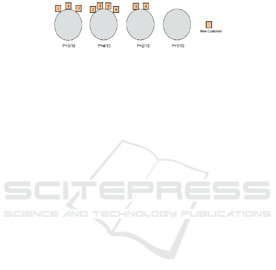
Figure 1: The Chinese Restaurant Process. Boxes represent the customers. Circles are the tables.
where C is the corresponding normalization constant.
h
r
represents the spatial resolution parameter which
affects the smoothing and connectivity. It is chosen
depending on the size of the object. h
m
is the resolu-
tion parameter of the motion feature which affects the
number of modes. It should be kept low if the vari-
ance of the state space is low. k(x) is the common
profile used in both two domains with the employed
kernel bandwidths h
r
and h
m
. We have to set only the
bandwidth parameters h = (h
r
, h
m
). Controlling the
sizes of the kernels determines the resolution of the
mode detection. Because of the variant object sizes
in 3D point cloud data, the mean-shift method tends
to generate over- and under-segmentations. However,
it is still a powerful mode seeking algorithm which
successfully performs as the first step of our proposed
hybrid method.
4.2 Chinese Restaurant Process
The ddCRP method presented in the following sub-
section is based on the Chinese Restaurant Process
(CRP) (Pitman et al., 2002), a hierarchical non-
parametric Bayesian clustering model originally pro-
posed for linguistic analysis and population genetics.
The CRP is typically introduced as a distribution over
partitions of data. For the generative process of a
CRP, a restaurant with a countably infinite number of
circle tables is imagined. Costumers enter the restau-
rant one by one. Either a customer takes a seat at a
table with a probability proportional to the number of
people already seated at that table, i.e. he is more
likely to sit at a table with many customers than with
few, or the customer takes a seat at a new empty table
with a probability proportional to a scaling parameter
α. Figure (1) illustrates a simple example of how the
customers choose the tables in a random process. The
first customer walks into the restaurant and sits at the
first table. The tenth customer enters the restaurant
and sits at one of the three tables (which have previ-
ously been chosen by the other nine customers) with
a probability proportional to the number of people al-
ready sitting at that table (the probabilities are written
below the tables) or sits at the unoccupied new table
with a probability proportional to a scaling parame-
ter. After all customers have entered the restaurant
and have been seated at a table, the resulting seating
plan of costumers provides the clustering of data. Al-
though it is described sequentially, the CRP is an ex-
changeable model, which means that the order of ob-
served data (or customers coming into the restaurant)
does not affect the posterior distribution. This does
not hold for point cloud data because the coordinates
of grid cells need to be considered to obtain contigu-
ous object segments.
4.3 Distance Dependent Chinese
Restaurant Process
The distance dependent Chinese Restaurant Process
(ddCRP) was introduced to model random partitions
of non-exchangeable data. It defines a distribution
over partitions indirectly via distributions over links
between data points. This leads to a biased clustering,
which means that each observed data point is more
likely to be clustered with other data that is near in an
external sense. For a naive example, considering time
series data, points closer in time are more likely to be
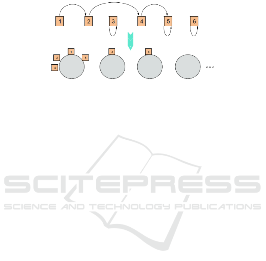
grouped together. Speaking in CRP terms, customers
are linked to other customers instead of tables, which
is shown in Figure (2). The seating plan probability is
described in terms of the probability of a customer sit-
ting with each of the other customers. The allocation
of customers to tables is a by-product of this represen-
tation. If two customers are reachable by a sequence
of interim customer assignments, then they sit at the
same table.
For the task of 3D point cloud data segmentation,
a restaurant represents each spatially extracted blob
from the pre-processing step; tables denote the seg-
ments, or objects, in the blob on inquiry and cus-
tomers are grid cells belonging to the blob.
A grid cell gr
t,i
in the time frame t has a link vari-
able c
i
which links to another cell gr
t, j
or to itself ac-
cording to the distribution below,
A Hybrid Method Using Temporal and Spatial Information for 3D Lidar Data Segmentation
165
(a)
Figure 2: The distance dependent Chinese Restaurant Process. It links customers to other customers, instead of tables. For
3D Lidar data, tables denote the segments in the blob on inquiry and customers are grid cells belonging to the blob.
p(c
i
= j|A, α) ∝
(
A
i j
if i 6= j,
α if i = j.
(6)
where the affinity A
i j
= f (d
i j
) depends on a spatial
distance d
i j
between the centers of mass of cells and
a decay function f (d). The decay function reflects
how the distances between grid cells affect the result-
ing distribution over partitions of the blob. We use a
window decay function f (d) = 1[d < a], which con-
siders grid cells that are at most a distance a away
from the center of mass of the current grid cell. The
spatial distance supports the discovery of connected
segments. Grid cells link together with a probability
proportional to A
i j
or cell gr
t,i
can stay alone and link
itself with a probability proportional to the scaling pa-
rameter α. It is shown in (Tuncer and Schulz, 2016b)
that larger α values favor partitions with more clus-
ters. Nearby cells are assigned to the same segment
if and only if they are in the same connected compo-
nent built by the grid cell links. The method enforces
the constitution of spatially connected segments. The
overall generative process can be summarized as fol-
lows:
1. For each grid cell gr
i
, sample its link assignment
c
i
v ddCRP(A, α)
2. Assign the customer links c
i
to the cluster assign-
ments z
i
. Then draw parameters θ
s
v G
0
for each
cluster.
3. For each grid cell, sample data x
i
v F(θ
s
) inde-
pendently. The s represents a segment in the blob.
The base distribution G
0
defines the mixture model
of the extracted clusters. It is selected as a con-
jugate prior of the data generating distribution with
Θ =
µ
0
, σ
2
0
. The F(θ
s
) is a Gaussian distribution
with θ
s
=
µ
s
, σ
2
. The state vector of a grid cell is
x
T
t
= [x
m
, x
r
], where x
m
is the one dimensional move-
ment direction of the grid cell and x
r
is its estimated
center of mass location in x and y directions. As the
nearby grid cells are probabilistically linked accord-
ing to x
r
by using Equation (6), the estimated motion
features x
m
are sampled according to the cell assign-
ments as the generative process described above.
4.4 Posterior Inference
Objects in spatially extracted blobs can be found by
a posterior inference. We explain how the ddCRP
framework determines the clusters, which represent
different objects, in a blob based on posterior infer-
ence. The key problem of inference is to compute
the posterior distribution of latent variables condi-
tioned on the spatial and temporal features. Due to
the huge combinatorial number of possible grid cell
layouts, it is intractable to evaluate the posterior prob-
ability directly. Therefore we make use of Gibbs sam-
pling (Geman and Geman, 1984) for the inference.
Gibbs sampling iteratively samples each latent vari-
able c
i
conditioned on the other latent variables c
−i
and the given state vector x as shown in the Equa-
tion (7) below,
p(c
i
|c
−i
, x, Ω) ∝ p(c
i
|A, α) p (x|z (c) , Θ) (7)
where Ω =
{
A, α, Θ
}
. The A is the affinity term, α
denotes the scaling factor, and Θ is the base distri-
bution. All these terms are explained in the previous
sub-section 4.3. The first term of Equation (7) is the
s-ddCRP prior given in Equation (6). The second one
is the likelihood, which is factorized according to the
cluster index as follows,
p(x|z (c), Θ) =
S
∏
s=1
p
x
z(c)=s
|Θ
(8)
ICINCO 2017 - 14th International Conference on Informatics in Control, Automation and Robotics
166

where x
z(c)=s
represents the state vectors of grid cells
assigned to the same segment s, and S denotes the
number of segments in a spatially extracted blob.
This factorization allows us to apply a block-wise
sampling because the algorithm does not need to re-
evaluate terms which are unaffected as the sampler
reassigns c
i
. Unless the cluster structure changes,
cached likelihood computations of previous iterations
can be used. Observations at each cluster are sam-
pled independently by using the parameters drawn
from the base distribution G
0
. The computation of
the marginal probability is given in Equation (9).
p
x
z(c)=s
|Θ
=
Z
∏
i∈z(c)=s
p(x
i
|θ)
!
p(θ|Θ)dΘ
(9)
Here i denotes the indices assigned to the segment
s and the Θ is the parameters of the base distribu-
tion G
0
. Selecting the conjugate p(x
i
|θ) and G
0
en-
ables the marginalization of θ. Then Equation (9)
can be computed analytically (Gelman et al., 2003).
The sampling algorithm explores the space of possi-
ble clusters in each spatially extracted blob by reas-
signing links c
i
. If c
i
is the only link connecting two
clusters, they split after the reassignment. When there
are other alternative links connecting those clusters,
the partitions of data stay unchanged. Reassigning the
link c
i
might newly connect two clusters as well. The
sampler considers how the likelihood is affected by
removing and randomly reassigning the cell links. It
needs to consider the current link c
i
and all its con-
nected cells, because if a cell gr
i
connects to a differ-
ent cluster, then all cells which are linked to it also
move to that cluster.
The Gibbs sampler explores the space of possible
segmentations with these reassignments. It computes
all cases which change the partition layout. Assuming
the cluster indices a and l joined to cluster d in a spa-
tially extracted blob, then a Markov chain is specified
as below:
p(c
i
|c
−i
, x, Ω) ∝
(
p(c
i
|A, α)Λ (x, z, Θ) if a ∪ l,
p(c
i
|A, α) otherwise,
(10)
where
Λ (x, z, Θ) =
p
x
z(c)=d
|Θ
p
x
z(c)=a
|Θ
p
x
z(c)=l
|Θ
(11)
The sampler generates different segmentation hy-
potheses and decides on the most probable ones by us-
ing temporal and spatial features together. The mean
value of the smoothed velocity vectors of grid cells
belonging to the same object can be assigned as a
motion feature of that object for tracking (Tuncer and
Schulz, 2016a).
5 EXPERIMENTAL RESULTS
The proposed method was evaluated on the real world
KITTI tracking data set (Geiger et al., 2012; Fritsch
et al., 2013; Geiger et al., 2013). That was recorded
using a Velodyne HDL-64D Lidar sensor and a high
precision GPS/IMU inertial navigation system. The
Lidar sensor has a frame rate of 10 Hz, a 360 degree
horizontal field of view and it produces approximately
1.1 million point measurements per second. We tested
the methods with KITTI tracking data set which con-
sists of more than 42,000 3D bounding box labels on
roughly 7,000 frames across 21 sequences. One of
these sequences is used to select parameters and the
remaining 20 sequences are used for evaluation. Es-
timated grid cell velocities are transformed to one-
dimensional movement directions. We set the reso-
lution parameter of the motion feature as h
m
= 0.5.
For an 8-neighborhood, the spatial resolution param-
eter is chosen as h
r
= 1. For the ddCRP part of the
proposed method, larger α values bias the algorithm
towards more clusters so we set α = 10
−4
(Tuncer and
Schulz, 2016b). The ddCRP sampler is run with 20 it-
erations for each extracted blob.
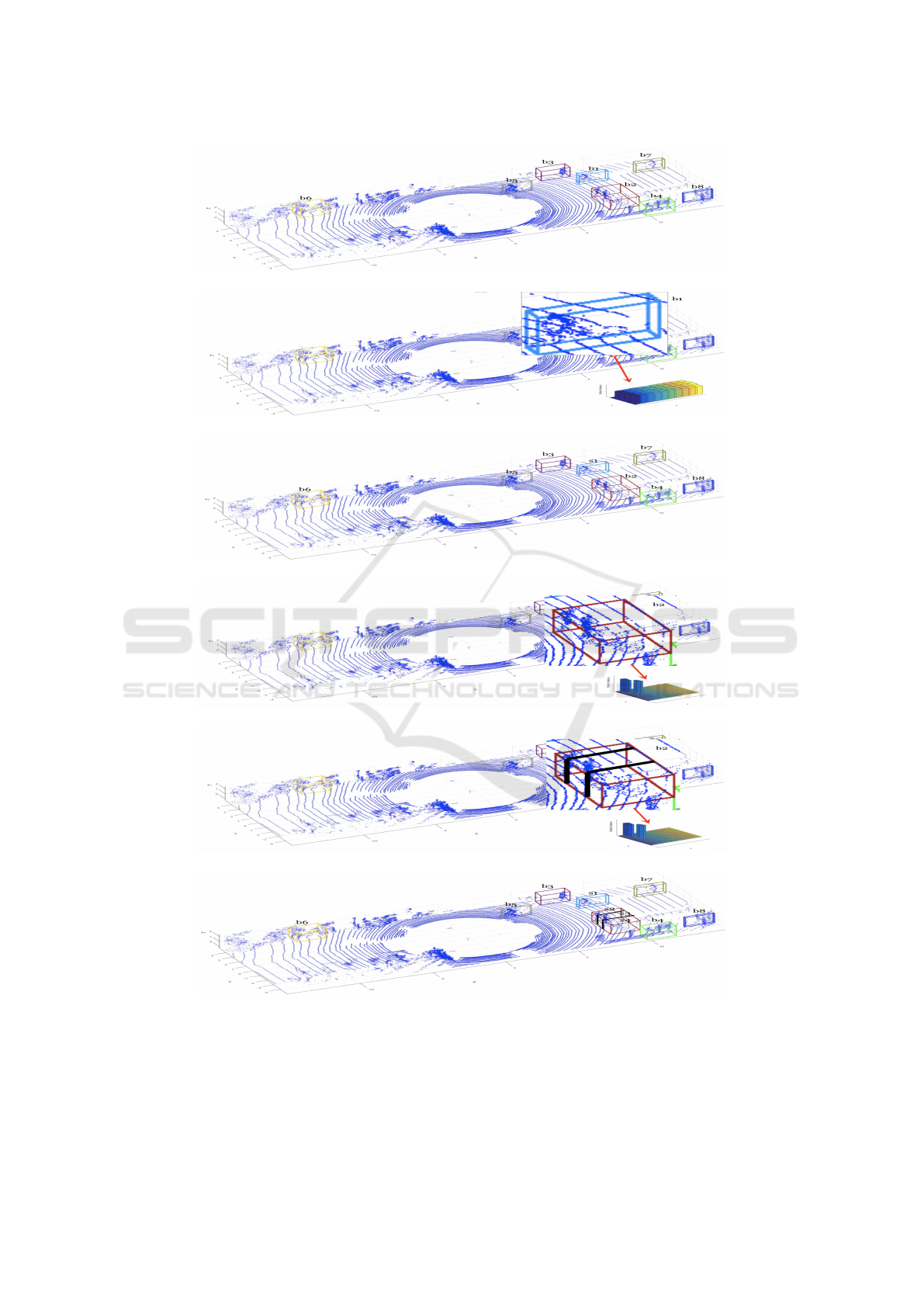
Figure (3) shows how the proposed hybrid method
runs for the segmentation of 3D Lidar data. Within a
time frame t, the blobs are spatially extracted from
the scene as shown in Figure (3)(a). They are rep-
resented by 3D boxes and named as b1, b2, .., b8. In
Figure (3)(b), the blob b1 is on query. The mean-
shift method seeks for the number of modes in the
state space of blob b1. The mean-shift algorithm de-
termines whether the blob on query might consist of
one object or multiple objects. Since the mean-shift
algorithm finds one mode in the state space, the hy-
brid method does not jump to the ddCRP level. The
blob b1 therefore remains the same and it is assigned
as a segment s1 as illustrated in Figure (3)(c). The
next blob b2 is on query in the Figure (3)(d). The
mean-shift method seeks for the number of modes in
the state space of the blob b2. It finds multiple modes
in the feature space. This means that the blob b2 is
under-segmented. Then the ddCRP method performs
the final partition on the blob b2 as illustrated in Fig-
ure (3)(e). The blob b2 is divided into three clusters,
which represent segments, or different objects. These
clusters are assigned as the segments s2, s3 and s4
as shown in Figure (3)(f). This procedure iteratively
continues while searching each blob in the scene at
A Hybrid Method Using Temporal and Spatial Information for 3D Lidar Data Segmentation
167
(a)
(b)
(c)
(d)
(e)
(f)
Figure 3: (a) Blobs are spatially extracted from the scene. The blobs are represented by 3D boxes and named such as
b1, b2, ...b8. (b) The mean-shift method seeks for the number of modes in the state space of blob b1. (c) Because the mean-
shift algorithm finds only one mode in the state space, the blob b1 remains the same and it is assigned as a segment s1. (d)
The next blob b2 is on query by the mean-shift method. (e) The mean-shift algorithm finds multiple modes in the feature
space of b2. Therefore the ddCRP method generates the final partition on the under-segmented blob b2 and splits up the blob
into three clusters. (f) These clusters are assigned as the segments s2, s3 and s4.
ICINCO 2017 - 14th International Conference on Informatics in Control, Automation and Robotics
168

each time frame. After the hybrid method has been
applied to each blob in a time frame, the algorithm
outputs the segmented scene.
The KITTI dataset has been used to evaluate track-
ing and object detection in the literature rather than
evaluating segmentation performances. The proposed
segmentation method is therefore evaluated using a
similar procedure described in (Held et al., 2016). For
the evaluation, the best matching segment is assigned
to each ground-truth bounding box. For each ground
truth box gt, the set of non-ground points P
gt
within
this box is identified. Then we assign the points P
s
to the segment s. The best matching segment to this
ground truth gt is found with Equation (12).
s = argmax
s
0
| P
s
0
∩ P
gt
| (12)
After the best matching segment is assigned to the
ground truth gt, Equation (13) is used as an evalua-
tion metric.
E =
1
N
∑
gt
1
k
P
s
∩ P
gt
k
k
P
s
k
< τ
s
(13)
where 1 is an indicator function which is 1 if the input
is true and 0 otherwise. The τ
s
is a constant threshold.
Table 1: Segmentation accuracies.
Method % Errors
Spatial Only 13.8
Mean-shift 12.7
s-ddCRP (Tuncer and Schulz, 2016b) 9.4
Hybrid 9.1
ddCRP (Tuncer and Schulz, 2015) 8.9
Table (1) shows the segmentation accuracies for the
given methods. The proposed hybrid method pro-
vides better accuracy compared to the s-ddCRP seg-
mentation approach (Tuncer and Schulz, 2016b). The
s-ddCRP method uses a priori coming sequentially
from the previous time frames and clusters the grid
cells agglomerative into super grid cells. These super
grid cells make the s-ddCRP algorithm more prone
to segmentation errors. Because of stationary under-
segmented objects, which do not have temporal cues,
and the group of nearby pedestrians moving in the
same direction, the error rate stays around 9%. A clas-
sification module might improve these results, and,
thus, is part of our future work. In addition we
plan to provide detailed statistical analyses to demon-
strate the significance of the improvement. Due to
the variant object sizes in 3D point cloud data, the
mean-shift method tends to generate over- and under-
segmentations, which results in a high error rate as
shown in Table (1). However, it is quite successful as
the first step of our proposed hybrid method on deter-
mining whether the feature space of the blobs consists
one or more modes.
(a)
Figure 4: The averaged computation time comparisons of
the mean-shift, hybrid, s-ddCRP and ddCRP methods. Al-
gorithms are implemented in Matlab.
Figure (4) compares the averaged computation time
of the mean-shift, hybrid, s-ddCRP and ddCRP meth-
ods. According to the computational complexity
given in the Figure (4), the hybrid method’s averaged
computational time decreases below the scanning pe-
riod of the Lidar scanner, which is 100 ms, making
the algorithm able to run in real time.
6 CONCLUSION
We proposed a hybrid method for the segmentation of
3D point cloud data which uses the mean-shift and dd-
CRP approaches. The proposed framework benefits
from the joint evaluation of geometrical and temporal
features to resolve ambiguities in complex dynamic
scenarios and to overcome the under-segmentation
problem of moving objects, i.e., assigning multiple
objects to one segment. For example, pedestrians of-
ten walk close to static objects so they are spatially
segmented together with their nearby objects. After
the motion field of the environment is estimated in one
dimensional movement directions and the segmenta-
tion blobs are spatially extracted from the scene, the
mean-shift seeks the number of possible objects in the
state space of each blob. If the mean-shift algorithm
determines an under-segmented blob, the ddCRP per-
forms the final partition in this blob. Otherwise, the
queried blob remains the same and it is assigned as
a segment. The proposed framework outputs a par-
titioning of the points in each time frame into dis-
joint segments, where each segment refers a single
object. Compared to the s-ddCRP and ddCRP seg-
mentation methods, incorporating the mean-shift and
ddCRP algorithms reduces the computational time re-
quirements of the system, which makes the algorithm
able to run in real time while having similar seg-
mentation accuracies. The autonomous vehicles’ sys-
tems segment the scene at the beginning of their per-
A Hybrid Method Using Temporal and Spatial Information for 3D Lidar Data Segmentation
169

ception pipeline so errors in segmentation propagates
throughout all the system. Better segmentation accu-
racy therefore improves other aspects of the system
such as tracking.
As future work, we plan to provide a detailed sta-
tistical analysis such as standard deviation to demon-
strate the significance of the improvement on segmen-
tation. Also, showing the effect of segmentation accu-
racy on object tracking would be useful to reveal how
the under-segmentation problem effects the whole ob-
ject recognition system of an autonomous vehicle.
The presented method does not benefit from the se-
quential nature of the problem. Adding a posterior
inference using prior knowledge from previous time
steps would speed up the overall system. The prior
knowledge obtained by the mean shift method could
also be used for this purpose.
Sub-sampling of 3D Lidar data by mapping indi-
vidual point measurements to an occupancy grid rep-
resentation and reduction of the motion estimation
into one dimension is sufficient to successfully dis-
criminate moving objects from their neighbors such
as buildings or parked cars. However, because of
stationary under-segmented objects and the group of
pedestrians moving in the same direction, the er-
ror rate stays around 9%. Exploiting an appearance
model together with the features of the grid represen-
tation would help to detect stationary nearby objects
and to separate each pedestrian in a group moving to-
wards the same direction. Also, this error rate en-
courages us to integrate a classification module as a
future work. Adding semantic cues would resolve the
under-segmentation problem of stationary nearby ob-
jects and, thus, improve the general segmentation ac-
curacy.
In addition, instead of estimating the motion of
the whole scene at each time step, the system might
decide to estimate only informative parts of the envi-
ronment by using semantic information. This could
further decrease the computational costs of the seg-
mentation and tracking components.
The detection of object classes would also be very
useful for the segmentation and tracking steps. To ob-
tain temporal information from the scene, applying
an iterative closest point approach would be interest-
ing instead of tracking each grid cell on an occupancy
grid. We intend to compare the performance of our
method with other novel algorithms proposed in the
literature.
ACKNOWLEDGEMENTS
We acknowledge the support by the EU’s Seventh
Framework Programme under grant agreement no.
607400 (TRAX, Training network on tRAcking in
compleX sensor systems) http://www.trax.utwente.nl/
REFERENCES
Azim, A. and Aycard, O. (2012). Detection, classification
and tracking of moving objects in a 3d environment.
In Intelligent Vehicles Symposium (IV), 2012 IEEE,
pages 802–807. IEEE.
Bar-Shalom, Y. (1987). Tracking and data association.
Academic Press Professional, Inc.
Blei, D. M. and Frazier, P. I. (2011). Distance dependent
chinese restaurant processes. The Journal of Machine
Learning Research, 12:2461–2488.
Choi, J., Ulbrich, S., Lichte, B., and Maurer, M. (2013).
Multi-target tracking using a 3d-lidar sensor for au-
tonomous vehicles. In Intelligent Transportation
Systems-(ITSC), 2013 16th International IEEE Con-
ference on, pages 881–886. IEEE.
Comaniciu, D. and Meer, P. (2002). Mean shift: A robust
approach toward feature space analysis. IEEE Trans-
actions on pattern analysis and machine intelligence,
24(5):603–619.
Douillard, B., Underwood, J., Kuntz, N., Vlaskine, V.,
Quadros, A., Morton, P., and Frenkel, A. (2011).
On the segmentation of 3d lidar point clouds. In
Robotics and Automation (ICRA), 2011 IEEE Inter-
national Conference on, pages 2798–2805.
Fritsch, J., Kuhnl, T., and Geiger, A. (2013). A new per-
formance measure and evaluation benchmark for road
detection algorithms. In Intelligent Transportation
Systems-(ITSC), 2013 16th International IEEE Con-
ference on, pages 1693–1700. IEEE.
Fukunaga, K. and Hostetler, L. (1975). The estimation of
the gradient of a density function, with applications in
pattern recognition. IEEE Transactions on informa-
tion theory, 21(1):32–40.
Geiger, A., Lenz, P., Stiller, C., and Urtasun, R. (2013).
Vision meets robotics: The kitti dataset. International
Journal of Robotics Research (IJRR).
Geiger, A., Lenz, P., and Urtasun, R. (2012). Are we
ready for autonomous driving? the kitti vision bench-
mark suite. In Computer Vision and Pattern Recogni-
tion (CVPR), 2012 IEEE Conference on, pages 3354–
3361. IEEE.
Gelman, A., Carlin, J. B., Stern, H. S., and Rubin, D. B.
(2003). Bayesian data analysis. Chapman and
Hall/CRC Texts in Statistical Science.
Geman, S. and Geman, D. (1984). Stochastic relaxation,
gibbs distributions, and the bayesian restoration of im-
ages. IEEE Transactions on pattern analysis and ma-
chine intelligence, (6):721–741.
Held, D., Guillory, D., Rebsamen, B., Thrun, S., and
Savarese, S. (2016). A probabilistic framework for
ICINCO 2017 - 14th International Conference on Informatics in Control, Automation and Robotics
170

real-time 3d segmentation using spatial, temporal, and
semantic cues. In Proceedings of Robotics: Science
and Systems.
Himmelsbach, M. and Wuensche, H.-J. (2012). Tracking
and classification of arbitrary objects with bottom-
up/top-down detection. In Intelligent Vehicles Sym-
posium (IV), 2012 IEEE, pages 577–582. IEEE.
Klasing, K., Wollherr, D., and Buss, M. (2008). A clus-
tering method for efficient segmentation of 3d laser
data. In Robotics and Automation, 2008. ICRA 2008.
IEEE International Conference on, pages 4043–4048.
IEEE.
Montemerlo, M., Becker, J., Bhat, S., Dahlkamp, H., Dol-
gov, D., Ettinger, S., Haehnel, D., Hilden, T., Hoff-
mann, G., Huhnke, B., et al. (2008). Junior: The
stanford entry in the urban challenge. Journal of field
Robotics, 25(9):569–597.
Moosmann, F., Pink, O., and Stiller, C. (2009). Segmen-
tation of 3d lidar data in non-flat urban environments
using a local convexity criterion. In Intelligent Vehi-
cles Symposium, 2009 IEEE, pages 215–220. IEEE.
Morton, P., Douillard, B., and Underwood, J. (2011). An
evaluation of dynamic object tracking with 3d lidar.
In Proc. of the Australasian Conference on Robotics
& Automation (ACRA).
Petrovskaya, A. and Thrun, S. (2009). Model based vehicle
detection and tracking for autonomous urban driving.
Autonomous Robots, 26(2-3):123–139.
Pitman, J. et al. (2002). Combinatorial stochastic processes.
Technical Report 621, Dept. Statistics, UC Berkeley,
2002. Lecture notes for St. Flour course.
Teichman, A., Levinson, J., and Thrun, S. (2011). Towards
3d object recognition via classification of arbitrary ob-
ject tracks. In Robotics and Automation (ICRA), 2011
IEEE International Conference on, pages 4034–4041.
IEEE.
Tuncer, M. A. C¸ . and Schulz, D. (2015). Monte carlo based
distance dependent chinese restaurant process for seg-
mentation of 3d lidar data using motion and spatial
features. In Information Fusion (FUSION), 2015 18th
International Conference on, pages 112–118. IEEE.
Tuncer, M. A. C¸ . and Schulz, D. (2016a). Integrated object
segmentation and tracking for 3d lidar data. In Pro-
ceedings of the 13th International Conference on In-
formatics in Control, Automation and Robotics - Vol-
ume 2: ICINCO, pages 344–351.
Tuncer, M. A. C¸ . and Schulz, D. (2016b). Sequential dis-
tance dependent chinese restaurant processes for mo-
tion segmentation of 3d lidar data. In Information Fu-
sion (FUSION), 2016 19th International Conference
on, pages 758–765. IEEE.
Urmson, C., Anhalt, J., Bagnell, D., Baker, C., Bittner, R.,
Clark, M., Dolan, J., Duggins, D., Galatali, T., Geyer,
C., et al. (2008). Autonomous driving in urban envi-
ronments: Boss and the urban challenge. Journal of
Field Robotics, 25(8):425–466.
A Hybrid Method Using Temporal and Spatial Information for 3D Lidar Data Segmentation
171
