
Modelling and Optimization of the Operation of a Multiple Tank Water
Pumping System
Roberto Sanchis and Ignacio Pe
˜
narrocha
D. Enginyeria de Sistemes Industrials i Disseny, University Jaume I, Castell
´
o, Spain
Keywords:
Pumping Optimization, Electric Tariff, Pumping Scheduling.
Abstract:
This paper studies the optimization of the operation of a water supply pumping system by means of standard
solvers. The system consists of several tanks that supply the water to several districts in a town. Each tank can
be filled from several wells through a hydraulic system that can be reconfigured by means of several valves.
The automatic operation of the system tries to determine which valves and pumps must be active at each
instant in order to minimise the operation cost, taking into account the tariff periods. The main constraints
are the maximum and minimum volumes of the tanks. A mathematical model of the problem is proposed in
order to formulate, in matrix form, the cost index and the constraints, to be able to use standard solvers as
Mosek. A basic optimization problem is proposed, that only imposes the constraints of the finite volume of
the tanks. The result of this basic problem tends to produce a large number of pump and valve commutations,
that is not adequate in practice. To solve this problem, two alternatives are proposed: to include the number
of commutations in the cost index, and to add as a constraint the maximum number of commutations. Both
approaches lead to an adequate result, but the second one is easier to use, as the number of commutations can
be fixed in an explicit way. An example of a real water supply system is analysed to demonstrate the validity
of the approach, using Yalmip as parser and Mosek as solver.
1 INTRODUCTION
An important cost in the operation of water supply
systems are the energetic cost associated to the pump-
ing system. Water consumers receive the water from
supply tanks that are filled up from wells. The opera-
tion cost depends on the instants during the day when
the pumps are working, since the electric tariff varies
along the day, following predefined tariffing periods.
The work (Ormsbee and Lansey, 1994) presents
a review of different approaches to the optimization
of water pumping systems, that depend on the con-
figuration of the system and the mathematical models
used. For the problem of filling the main tanks, that is
the objective of this paper, the most commonly used
model is the mass-balance one. In most of the works,
the cost function takes into account the energy con-
sumed, but not the tariffing periods when that energy
is consumed. On the other hand, the decision vari-
ables are usually the fraction of operation time of each
pump in some predefined intervals. Other indirect de-
cision variables have also been proposed (as the tank
volumes), but the relation to the cost index and to the
final decision (the pumps and valves commands) is
too complex for the case we are studying.
In a more recent work, (Bunn and Reynolds,
2009), different approaches are reviewed, focusing
on real-time dynamic optimization technologies and
data-mining techniques to improve energy efficiency.
This work describes a commercial optimization soft-
ware for water distribution systems that can solve the
problem we are facing in this paper and other more
complex ones, but the details about the algorithms
used are not given.
Most of the recent works, as (Savic et al., 1997),
(Powell and McCormick, 2004), (Martinez et al.,
2007) , (Sotelo et al., 2002) or (Wegley et al., 2000)
use complex models of the hydraulic systems, and
are based on complex optimization algorithms, as ge-
netic algorithms, particle swarm or simulated anneal-
ing. Those approaches have a high computer cost,
especially for large systems.
In this paper a simple model is used in order to
formulate an optimization problem that can be solved
with standard solvers, with a low computer cost.
In (Pasha and Lansey, 2009), a linear program-
ming approach is used for the optimization of the
pumps operation, but is only applicable for a single
144
Sanchis, R. and Peñarrocha, I.
Modelling and Optimization of the Operation of a Multiple Tank Water Pumping System.
DOI: 10.5220/0006471501440154
In Proceedings of the 14th International Conference on Informatics in Control, Automation and Robotics (ICINCO 2017) - Volume 1, pages 144-154
ISBN: 978-989-758-263-9
Copyright © 2017 by SCITEPRESS – Science and Technology Publications, Lda. All rights reserved

tank system. In (Fang et al., 2010), the problem of op-
timization of pumps operation in a multi tank system
is studied using complex genetic algorithms.
In (Ormsbee et al., 2009) three different explicit
formulations of the optimal pump scheduling problem
are presented. It takes into account the electric tar-
iff, but the decision variables define the start and stop
times of the different pumps in the system. The result-
ing optimization problem needs to be solved by non
linear algorithms, genetic algorithms, or semi heuris-
tic ad-hoc algorithms. This discrete explicit formula-
tion is not directly applicable if the system has some
valves that can reconfigure the network. In that case
is not sufficient to decide which pumps are started
or stopped at which time, but also the switching of
the valves, that changes the resulting inlet flow to the
tanks for a given pumps state. Furthermore, our ob-
jective is to use standard solvers to deal with the op-
timization problem. For that reason, in this paper, the
decision variables are explicit, but consist of the com-
bination of pumps and valves that must be active at
each instant, from the set of possible combinations.
The mathematical formulation proposed allows to use
standard parsers (as Yalmip) and solvers (as Mosek or
CBC), to solve the optimization problem.
In section II the problem of pumping system opti-
mal operation is described. In section III the mathe-
matical model of the problem is developed. In section
IV the basic optimization problem, derived from the
mathematical problem, is formulated. A more com-
plex optimization problem is formulated in section V
to reach more practical solutions, with a reduced num-
ber of pump commutations. Section VI shows the ap-
plication to a real pumping system and section VII
summarizes the main conclusions.
2 DESCRIPTION OF THE
PROBLEM
This paper deals with the problem of optimizing the
operation of a water pumping system a predefined
structure, with several wells and pumps, several tanks
and several ducts and valves. The objective of the
optimization is the minimization of the overall op-
erational cost. This cost is related to the individual
pumping energetic cost of each well (kWh per cubic
meter) and, especially, to the electric tariff that es-
tablish a different price depending on the time. The
automatic control system must decide which valves
and which pumps should be operated at every time
along the day to minimize the cost while fulfilling
some constraints.
The main constraint is to serve from each tank the
required daily water flow. This flow is time varying
and uncertain, but it can be predicted because it fol-
lows an approximate daily pattern. The other impor-
tant constraint is due to the size of the tanks, each one
having a maximum and minimum level that should
not be violated.
Other secondary constraints that may apply in-
clude a maximum number of daily starts and stops of
each pump, or a minimum running time once a pump
is switched on. Other more complex restrictions could
be related to the concentration of some pollutants in
the different wells. For example, the nitrate concen-
tration may be too high in a given well, so that, that
water must be mixed with the one from another well
to fulfil a concentration requirement. The constraint
could then be a minimum mixing ratio. This last con-
straint could be time varying, as the concentration of
the wells may change with time.
3 MATHEMATICAL
MODELLING OF THE
PROBLEM
First of all, the pumping system is assumed to have N
p
pumps (one in each well), N
t
tanks and N
v
valves. The
valves are used to connect or disconnect the pumps to
the tanks. The total number of possible combinations
is 2
N
p
+N
v
, but not all the combinations are possible
in a given system. Let us define as N
c
the number
of valid combinations of valves and pumps. In or-
der to formulate mathematically the problem, a bi-
nary matrix, M
c
, of size N
c
× (N
p
+ N
v
), is defined,
where each row represents one of the valid combina-
tions, and where the corresponding elements take the
value 1 or 0 depending on the active or inactive state
of the valves and the pumps in that combination.
Along the paper, a simple example will be used
to illustrate the proposed approach. The considered
pumping system has N
p
= 2 wells (pumps), N
v
= 1
valve and N
t
= 2 tanks. The tank 1 can be filled from
pump 1, no matter the state of the valve (with a flow
of 200 m
3
/h), and from pump 2 if the valve 2 is open
(with an additional flow of 100 m
3
/h), while the tank
2 can only be filled from pump 2 if the valve is closed
(with a flow of 80 m
3
/h).
Taking into account the physical limitations de-
scribed above, the matrix that defines de N
c
= 6 valid
combinations of pumps and valves in this example is
shown in table 1. The value X means that the resulting
flows are the same if the valve is closed (0) or open
(1).
For each combination of valves and pumps, there
Modelling and Optimization of the Operation of a Multiple Tank Water Pumping System
145

Table 1: Possible combinations of simple example.
Comb V P
1
P
2
0 X 0 0
1 X 1 0
2 0 0 1
3 1 0 1
4 0 1 1
5 1 1 1
is a resulting outlet flow of each pump, and a resulting
inlet flow for each tank. This can be expressed by a
matrix of pump flows, F
P
, that has as many columns
as combinations, and one row per pump and a matrix
of tank inlet flows, F
T
, that has as many columns as
combinations, and one row per tank, i.e. the size of
matrices F
P
and F
T
are (N
p
×N
c
) and (N
t
×N
c
). In the
proposed example, the resulting flow matrices could
be (in m
3
/h):
F
P
=
0 200 0 0 200 200
0 0 80 100 80 100
(1)
F
T
=
0 200 0 100 200 300
0 0 80 0 80 0
(2)
For each combination there is a matrix that relates
the pump flows to the tank flows. For example, for
combination 5, the tank flows can be expressed as a
function of pump flows as
f
T
= M
5
f
P
=
1 1
0 0
200
100
=
300
0
(3)
The matrix that relates the flows is different for each
combination of pumps and valves. In the example the
matrices are:
M
0
= M
1
= M
2
= M
4
=
1 0
0 1
M
3
= M
5
=
1 1
0 0
Following the same procedure, a matrix P can be
formed with the electric power consumption of each
pump for each combination. The matrix has as many
columns as combinations, and one row per pump, i.e.
the size of matrix P is (N
p
× N
c
). In the proposed
example, the power matrix (in kW) is:
P =
0 20 0 0 20 20
0 0 10 12 10 12
(4)
In order to operate the water supply facility, the
automatic management system must decide which
one of those N
c
combinations has to be applied at each
instant of time. The natural objective is to minimize
the overall operation cost. In order to be able to for-
mulate the optimization problem, a variable taking in-
teger values from 0 to N
c
could be defined. However,
in order to formulate more easily the objective func-
tion as well as the constraints, a binary vector is pro-
posed to define the applied combination as a function
of time:
δ(t) ∈ {δ
1
,. .., δ
N
c
} (5)
with
δ
i
= [0 ··· 0
| {z }
i−1
1 0· ··0]
T
(6)
Therefore, the elements of δ(t) can only be 0 or 1,
and only one of the elements can be different from
zero (i.e. the sum of the elements is 1).
With these definitions, the vector that gathers the
inlet flows of the tanks at a given instant is simply the
product
f
T
(t) = F
T
δ(t),
the vector of output flow of the pumps is
f
P
(t) = F
P
δ(t),
while the vector of power consumptions of the pumps
is
p(t) = Pδ(t)
The matrix that relates the pump flows and the
tank flows can be expressed as a function of δ:
M(δ) =
δ
T
0 ·· · 0
0 δ
T
.
.
.
.
.
.
.
.
.
.
.
.
.
.
.
0
0 ·· · 0 δ
T
N
T
×N
T
N
c
·
M
0
(1,:)
M
1
(1,:)
.
.
.
M
N
c
(1,:)
M
0
(2,:)
.
.
.
M
N
c
(N
t
,:)
N
T
N
c
×N
p
(7)
With that definition,
f
T
(t) = M(δ(t)) f
P
(t) (8)
In order to compute the overall cost, the elec-
tric tariff must be taken into account. The tariff can
be expressed as a function that defines the price in
euro/kW h as a function of time, T
i
(t). Each pump
could have a different tariff, hence, we define a row
vector as:
T (t) =
T
1
(t) ·· · T
N
p
(t)
(9)
With this, the overall cost in a period of time can
be expressed (in euros ) as:
J =
1
3600
Z
T (t)Pδ(t)dt (10)
The equation of the tanks can be expressed as:
˙
V
j
= f
T, j
(t) − f o
j
(t) (11)
ICINCO 2017 - 14th International Conference on Informatics in Control, Automation and Robotics
146

where f
T, j
(t) and f o
j
(t) are the inlet and outlet flow
of tank j respectively. The equations of all the tanks
can be joined in matrix form
˙
V =
˙
V
1
···
˙
V
N
t
=
f
T,1
(t)
···
f i
T,N
t
−
f o
1
(t)
···
f o
N
t
= f
T
(t) − f o(t)
(12)
If the future output flow of each tank, f o(t), were
known, then the volume could be calculated accu-
rately. However, the future output flow is unknown
and, hence, a prediction
ˆ
f o(t) must be used. On the
other hand, the input flow can be expressed as a fun-
cion of δ(t), therefore, the equation used to estimate
the evolution of the volume of the tanks (in m
3
/s) is
˙
V =
1
3600
F
T
δ(t) −
ˆ
f o(t)
(13)
where the flows are in m
3
/h.
In order to obtain a tractable formulation of the
problem, the continuous time equations must be dis-
cretized. If we choose a constant discretizing period
h, the vector funcions T (t) and δ(t) would then be
changed by vectors of discrete signals T [k] = T (t =
kh) and δ[k] = δ(t = kh). δ(t) is assumed to maintain
a constant value during interval h, i.e. δ(t) = δ[k] for
k h <= t < (k + 1)h. Taking into account the units of
the variables, the cost index (in euros) could be ex-
pressed as:
J =
h
3600
∑
T [k]Pδ[k] (14)
The continuous time equation of the tanks must
also be discretized at period h. The discretized equa-
tion can be expressed as:
V [k + 1] = V [k] +
h
3600
F
T
δ[k] −
ˆ
f o[k]
(15)
where V [k] = V (t = k h) and
ˆ
f o[k] =
1
h
R
(k+1)h
kh
ˆ
f o(t)dt.
The main constraints are the maximum and min-
imum limits of the tank volums, therefore, the con-
straints can be formulated as
V
i,min
≤ V
i
[k] ≤ V
i,max
, i = 1,··· ,N
t
(16)
or in matrix form
V
min
≤ V[k] ≤ V
max
(17)
4 BASIC OPTIMIZATION
PROBLEM
The basic optimization problem consists of minimiz-
ing the cost of the energy while fulfilling the main
constraints of maintaining the volumes of all the tanks
inside their admissible range (between their minimum
and maximum values). An additional constraint must
be added in order to guarantee that the tanks finish the
day with the same volume they have started. Other-
wise, the solution will always finish the day with the
tanks completely empty.
Taking into account the equations introduced in
the previous sections, with the definition of vectors
δ[k], T [k], V [k] and
ˆ
f
o
[k], and taking a minimization
horizon, t
m
= k
m
h, the minimization problem can be
formulated as:
min
δ
h
3600
∑
k
m
k=1
T [k]Pδ[k]
s.t. V
min
≤ V (0)+
h
3600
∑
k
j=1
F
T
δ[ j] −
ˆ
f
o
[ j]
≤ V
max
∑
k
m
j=1
F
T
δ[ j] −
ˆ
f
o
[ j]
≥ 0
kδ[k]k = 1, δ[k] ∈ {0, 1}
k = 1,.. . ,k
m
(18)
This problem can be expressed in matrix form in a
more compact way by joining vectors δ[k] and T [k]
in some matrices of adequate sizes (∆
(k
m
N
c
×1)
and
T
(1×k
m
N
p
)
), and defining the following vectors and ma-
trices:
∆ =
δ[1]
.
.
.
δ[k
m
]
k
m
N
c
×1
(19)
T =
h
3600
T [1] · ·· T [k
m
]
1×k
m
N
p
(20)
P =
P 0 ·· · 0
0 P
.
.
.
.
.
.
.
.
.
.
.
.
.
.
.
.
.
.
0 ·· · 0 P
k
m
N
p
×k
m
N
c
(21)
F
k
=
F
T
F
T
·· · F
T
| {z }
k
0 ·· · 0
N
t
×k
m
N
c
(22)
I
k
=
0 ·· · 0
| {z }
(k−1)N
c
1 ·· · 1
| {z }
N
c
0 ·· · 0
(23)
ˆ
F
O
[k] =
k
∑
j=1
ˆ
f
o
[ j] (24)
Using these definitions, the minimization problem
can be formulated as:
Modelling and Optimization of the Operation of a Multiple Tank Water Pumping System
147

min
∆
TP∆ (25)
s.t.
F
k
∆ ≥ 3600
V
min
−V (0)
h
+
ˆ
F
O
[k], k = 1, ..., k
m
F
k
∆ ≤ 3600
V
max
−V (0)
h
+
ˆ
F
O
[k], k = 1, ..., k
m
F
k
m
∆ ≥
ˆ
F
O
[k
m
]
I
k
∆ = 1, k = 1,. .. ,k
m
∆[ j] ∈ {0, 1} j = 1,·· · ,k
m
N
c
The optimization problem (25) is a mixed inte-
ger one, where the decision variables are the elements
of vector ∆ that can only take values 0 or 1. The
number of decision variables is N
c
k
m
, and the num-
ber of constraints is (2N
c
+ 2N
t
+ 1)k
m
+ N
t
. For a
normal prediction horizon of 1 day, if a discretiz-
ing period of 1 minute is taken, the number of vari-
ables is 1440N
c
, and the number of constraints is
1440(2N
c
+ 2N
t
+ 1)+ N
t
, that can be very large even
for quite simple systems. Even if a longer perid of,
for example, 5 minutes is chosen, the number of vari-
ables is still large (288N
c
). Furthermore, the mixed
integer optimization is highly demanding in computer
resources, and the optimization should be run fre-
quently (not only once a day), to use the most up
to date output flow estimations. Therefore, in order
to reduce the complexity, we propose to use two dis-
cretizing periods, a short one for the first hours, h, and
a coarser one for the rest of the day, h
M
= Lh. Defin-
ing the shorter time horizon as t
m
= k
m
h, and the total
time horizon t
M
= t
m
+(k
M
−k
m
)Lh, the optimization
problem could be expressed as:
min
∆
h
3600
∑
k
m
k=1
T [k]Pδ[k] +
Lh
3600
∑
k
M
i=k
m
+1
T [i]Pδ[i]
s.t. V
min
≤ V (0)+
h
3600
∑
k
j=1
F
T
δ[ j] −
ˆ
f
o
[ j]
≤ V
max
k = 1,.. . ,k
m
V
min
≤ V (k
m
) +
Lh
3600
∑
k
i=k
m
+1
F
T
δ[i] −
ˆ
f
o
[i]
≤ V
max
k = k
m
+ 1,. .. , k
M
kδ[k]k = 1, δ[k] ∈ {0, 1}
k = 1,.. . ,k
M
(26)
where the size of matrix ∆ is now (k
M
) × N
c
, and
where
T [k] =
T (t = kh) i f k ≤ k
m
T (t = k
m
h +(k − k
m
)Lh) i f k
m
< k ≤ k
M
(27)
and where
ˆ
f o[k] =
(
1
h
R
(k+1)h
kh
ˆ
f o(t)dt i f k ≤ k
m
1
Lh
R
k
m
h+(k+1−k
m
)Lh
k
m
h+(k−k
m
)Lh
ˆ
f o(t)dt i f k
m
< k ≤ k
M
(28)
Using the same vectors and matrices defined previ-
ously (∆, P, I
k
), but of fize k
M
instead k
m
, and re-
defining matrix T as
T =
h
3600
T [1] · ··T [k
m
] T [k
m
+ 1]L· · · T[k
M
]L
1×k
M
N
p
(29)
and redefining matrix F
k
and
ˆ
F
O
[k] for k > k
m
as
F
k
=
F
T
··· F
T
| {z }
k
m
LF
T
··· LF
T
| {z }
k−k
m
0 ··· 0
N
t
×k
M
N
c
(30)
ˆ
F
O
[k] =
k
m
∑
j=1
ˆ
f
o
[ j] + L
k
∑
j=k
m
+1
ˆ
f
o
[ j] (31)
the optimization problem can be formulated as:
min
∆
TP∆
s.t.
F
k
∆ ≥ 3600
V
min
−V (0)
h
+
ˆ
F
O
[k], k = 1, .. .,k
M
F
k
∆ ≤ 3600
V
max
−V (0)
h
+
ˆ
F
O
[k], k = 1, .. .,k
M
F
k
M
∆ ≥
ˆ
F
O
[k
M
]
I
k
∆ = 1, k = 1,.. . ,k
M
∆[ j] ∈ {0, 1} j = 1, ·· · ,k
M
N
c
(32)
The number of decision variables in problem (32)
is N
c
k
M
, and the number os constraints is (2N
c
+
2N
t
+ 1)k
M
+ N
t
. For example, choosing a short dis-
cretizing period h = 5 minutes, k
m
= 36 (equivalent
to 3 hours), and a long period Lh = 20 minutes, with
k
M
= 99 (equivalent to 1 day total horizon), for a sys-
tem with N
c
= 10, and N
t
= 3, the number of variables
is 990, while the number of constraints is 2676.
The optimization problem (32) depends on the
prediction of the future flow demand
ˆ
f o[k], that is un-
certain. The prediction can be improved for the short
term as the output flow is measured on line. There-
fore, in order to obtain more accurate results, the op-
timization must be run periodically, so that, a less un-
certain flow prediction is used. For example, it could
be run every hour. In that case, only the values of
δ[k] obtained for the first hour would be applied, dis-
carding the rest. This is a usual strategy in predictive
control.
As we are enforcing a final volume equal than
the initial one, the result of the optimization depends
on the initial condition of the tanks, and the instant
of time during the day when the optimization is car-
ried out. In order to set a framework for compar-
ison purposes, the optimization will be assumed to
ICINCO 2017 - 14th International Conference on Informatics in Control, Automation and Robotics
148

be carried out at the instant when the cheapest pe-
riod ends, and the initial volumes are assumed to be
V (0) = 0.95V
max
, i.e. near the maximum. This con-
ditions reinforce the idea of maximizing water avail-
ability in case a problem occurs with any pump.
One drawback of this simple optimization is that it
tends to produce a large number of pumps and valves
commutations.
5 ADVANCED OPTIMIZATION
PROBLEM
The main drawback of the basic optimization problem
(32) is that the optimal solution tends to imply a large
amount of commutations, i.e. the pumps and valves
would be stopping and starting every few minutes.
This is a serious problem, since every start and stop
implies an energy waste and a reduction in the work-
ing life of hydraulic components. Therefore, the opti-
mization problem must be modified to achieve a low
number of commutations for the proposal to be use-
ful. There are two approaches for limiting the number
of commutations:
• To include in the cost index a term that depends on
the number of commutations. There are two dif-
ficulties: the formulation of the number of com-
mutations, and to decide the weight of this term
relative to the main cost index.
• To add some constraints to limit the number of
commutations. The constraints could relate to the
number of combination changes, or the number of
commutations in each pump or in each valve.
5.1 Formulation of Number of
Commutations
If we consider the number of commutations as the
number of changes in δ[k] along the optimization pe-
riod, we need an equation that expresses that number
of changes as a function of matrix ∆. If the following
matrices are defined:
I
+
N
=
N
z }| {
0 ·· · 0 1 0 ·· · 0
.
.
.
.
.
.
.
.
.
.
.
.
.
.
.
.
.
.
0
.
.
.
·· ·
.
.
.
1 0
0 ·· · ··· ··· 0 1
(k
M
−1)N×k
M
N
I
−
N
=
1 0 · ·· · ·· ··· 0
0 1
.
.
.
.
.
.
.
.
.
0
.
.
.
.
.
.
.
.
.
.
.
.
.
.
.
.
.
.
0 ·· · 0 1 0 ··· 0
| {z }
N
(k
M
−1)N×k
M
N
Y
N
= I
+
N
− I
−
N
The number of changes in δ[k] can be expressed as:
∆
T
Y
T
N
c
Y
N
c
∆ = sum(abs(Y
N
c
∆)) (33)
Another possibility is to consider the number of
commutations of the pumps. In order to obtain the ex-
pression of number of pump commutations, let us de-
fine matrix S
P
as a matrix with 1 or 0 defining which
pumps are active at each combination. In the case of
our example this matrix would be:
S
P
=
0 1 0 0 1 1
0 0 1 1 1 1
T
(34)
such that S
p
δ[k] is a vector with values 1 or 0 depend-
ing on the state of each pump. Defining matrix S as
S =
S
P
0 ··· 0
0 S
P
0 ··· 0
.
.
.
.
.
.
.
.
.
.
.
.
0 ·· · 0 S
P
N
p
k
M
×N
c
k
M
(35)
The overall number of pump commutations is
∆
T
S
T
Y
T
N
p
Y
N
p
S∆ = sum(abs(Y
N
p
S∆)) (36)
5.2 Modification of Cost Index
The first alternative to reduce the number of commu-
tations is to include the number of changes in the cost
index. In this case the optimization problem can be
formulated as:
min
∆
TP∆ + α∆
T
Y
T
Y∆ (37)
s.t.
F
k
∆ ≥ 3600
V
min
−V (0)
h
+
ˆ
F
O
[k], k = 1, ..., k
M
F
k
∆ ≤ 3600
V
max
−V (0)
h
+
ˆ
F
O
[k], k = 1, ..., k
M
F
k
M
∆ ≥
ˆ
F
O
[k
M
]
I
k
∆ = 1, k = 1,... ,k
M
∆[ j] ∈ {0, 1} j = 1,··· ,k
M
N
c
where Y = Y
N
c
if the number of changes in δ[k] is to
be minimized, and Y = Y
N
p
S if the number of pump
commutations is to be considered. The weighting fac-
tor α must be chosen carefully to find a compromise
Modelling and Optimization of the Operation of a Multiple Tank Water Pumping System
149

between minimization of the cost and the number of
commutations.
In order to add the expression of the number of
changes to the cost index in Yalmip, such that the
solvers can deal with it, instead of ∆
T
Y
T
Y ∆, the
equivalent expression sum(abs(Y∆)) is used.
5.3 Adding Constraints
The drawback of the previous approach is that the
result is highly dependent on the weighting factor α
used, and is not easy to predict the result in terms of
number of commutations as a function of α. The sec-
ond alternative tries to overcome this drawback. It
consists of adding new constraints to limit the number
of changes. The optimization problem would then be:
min
∆
TP∆ (38)
s.t.
F
k
∆ ≥ 3600
V
min
−V (0)
h
+
ˆ
F
O
[k], k = 1, ..., k
M
F
k
∆ ≤ 3600
V
max
−V (0)
h
+
ˆ
F
O
[k], k = 1, ..., k
M
F
k
M
∆ ≥
ˆ
F
O
[k
M
]
∆
T
Y
T
Y ∆ ≤ c
max
I
k
∆ = 1, k = 1,... ,k
M
∆[ j] ∈ {0, 1} j = 1,··· ,k
M
N
c
where again Y = Y
N
c
if the number of changes in δ[k]
is to be minimized, and Y = Y
N
p
S if the number of
pump commutations is to be considered. The constant
c
max
represents the maximum number of changes or
pump commutations in the overall optimization pe-
riod.
Again, in order to add the expression of the num-
ber of changes to the constraints in Yalmip, instead of
∆
T
Y
T
Y ∆, the equivalent expression sum(abs(Y ∆))
is used.
6 APPLICATION EXAMPLE
A real application example, obtained from a real wa-
ter supply facility, will be used to illustrate the pro-
posed approach. The considered pumping system has
N
p
= 3 wells (pumps), N
v
= 2 valves and N
t
= 3 tanks.
The tank 3 can be filled from pump 1, no matter the
state of the valves, or from pump 2, if the valve 2 is
open, or from pump 3, also if the valve 2 is open. The
tank 2 can only be filled from pump3 if the valve 2 is
closed and the valve 1 open. Finally, the tank 1 can
only be filled from pump 3 if both valves are closed.
The pump 1 and 3 can work simultaneously, but pump
2 can only operate if the other two are stopped.
Taking into account the physical limitations de-
scribed above, the matrix that defines de N
c
= 10 valid
combinations of pumps and valves is shown in table
2. Again, the X value represents that the flows do not
depend on the state of the valve.
Table 2: Valid combinations in the application example.
Comb V
1
V
2
P
1
P
2
P
3
0 X X 0 0 0
1 0 0 0 0 1
2 1 0 0 0 1
3 X 1 0 0 1
4 X 1 0 1 0
5 X X 1 0 0
6 0 0 1 0 1
7 1 0 1 0 1
8 X 1 1 0 1
9 X 1 1 1 0
For each combination of valves and pumps, there is
a resulting outlet flow of each pump, and a resulting
inlet flow for each tank, defined by the respective ma-
trices. The resulting flow matrices are (in m
3
/h):
F
P
=
0 0 0
0 0 80
0 0 100
0 0 120
0 100 0
200 0 0
200 0 80
200 0 100
200 0 120
200 100 0
T
(39)
F
T
=
0 0 0
80 0 0
0 100 0
0 0 120
0 0 100
0 0 200
80 0 200
0 100 200
0 0 320
0 0 300
T
(40)
For each combination there is a matrix that relates
the pump flows to the tank flows. For example, for
combination 6, the tank flows can be expressed as a
function of pump flows as
ICINCO 2017 - 14th International Conference on Informatics in Control, Automation and Robotics
150
f
T
= M
6
f
P
=
0 0 1
0 0 0
1 0 0
200
0
80
=
80
0
200
(41)
The matrix that relates the flows is different for
each combination of pumps and valves. In the exam-
ple the matrices are:
M
0
=
0 0 0
0 0 0
0 0 0
M
1
= M
6
=
0 0 1
0 0 0
1 0 0
M
2
= M
7
=
0 0 0
0 0 1
1 0 0
M
3
= M
4
= M
5
= M
8
= M
9
=
0 0 0
0 0 0
1 1 1
The matrix P defines the electric power consump-
tion of each pump for each combination. The matrix
has as many columns as combinations, and one row
per pump, i.e. the size of matrix P is (N
p
×N
c
). In the
proposed example, the power matrix (in kW) is:
P =
0 0 0
0 0 13
0 0 11
0 0 7
0 5 0
12 0 0
12 0 13
12 0 11
12 0 7
12 5 0
T
(42)
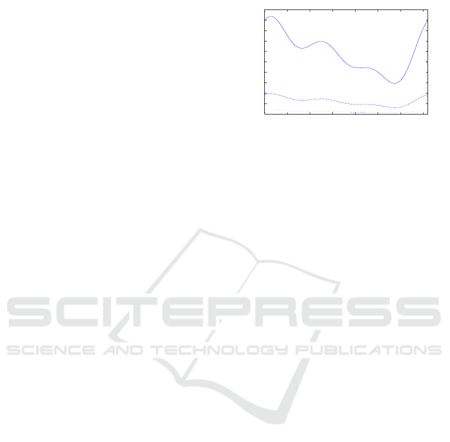
In order to perform the calculations, the outlet
flow of the tanks is estimated through a Fourier se-
ries from real data. The figure 1 shows the ouput flow
of the three tanks for one day, starting at 8 a.m.
The simple optimization problem (32) has been
solved with Matlab, using Yalmip as parser and
Mosek solver.
As we are enforcing a final volume equal than
the initial one, the result of the optimization depends
on the initial condition of the tanks, and the instant
of time during the day when the optimization is car-
ried out. In order to set a framework for compar-
ison purposes, the optimization will be assumed to
be carried out at the instant when the cheapest pe-
riod ends, and the initial volumes are assumed to be
0 200 400 600 800 1000 1200 1400
0
20
40
60
80
100
120
140
160
180
200
Estimated outlet flow of tanks 1, 2 and 3
Figure 1: Estimated outlet flow of tanks 1,2 and 3, in m
3
/h.
V (0) = 0.95V
max
, i.e. near the maximum. This con-
ditions reinforce the idea of maximizing water avail-
ability in case a problem occurs with any pump.
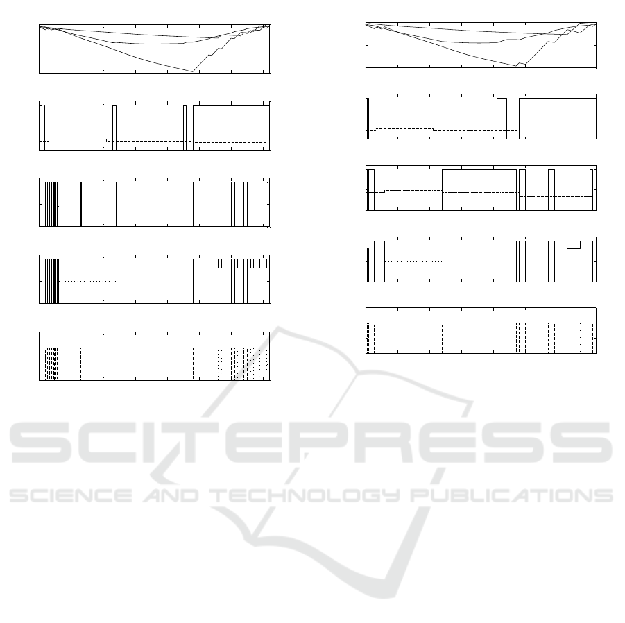
The figure 2 shows the result of the optimization
with h = 5 minutes, L = 4, k
m
= 60 and k
M
= 117, i.e.
5 hours at a period of 5 minutes, and 19 hour at a pe-
riod of 20 minutes. The optimum value is J = 17.22.
The figure shows the volumes in percentage, the flow
of the three pumps (with the timely price of the asso-
ciated tariff), and the state of the valves. The draw-
back of this approach is that the number of commuta-
tions in the day is quite high (56 pump commutations
and 28 valve commutations). The commutations are
especially frequent during the first 5 hours when the
period of discretization is smaller. If a period of h = 5
minutes is used for all the day, the number of com-
mutations is 120 for the pumps and 68 for the valves,
while the cost index is slightly lower J = 17.04.
If the number of changes in δ is considered in the
cost index, with a weighting factor α = 0.02, the re-
sult of the optimization (37) is shown in figure 3. The
number of pump commutations is 31, and the number
of valve changes is 14. The cost index is only slightly
higher then the case where the number of changes is
not included in the cost index, J = 17.26 (only the
energy cost).
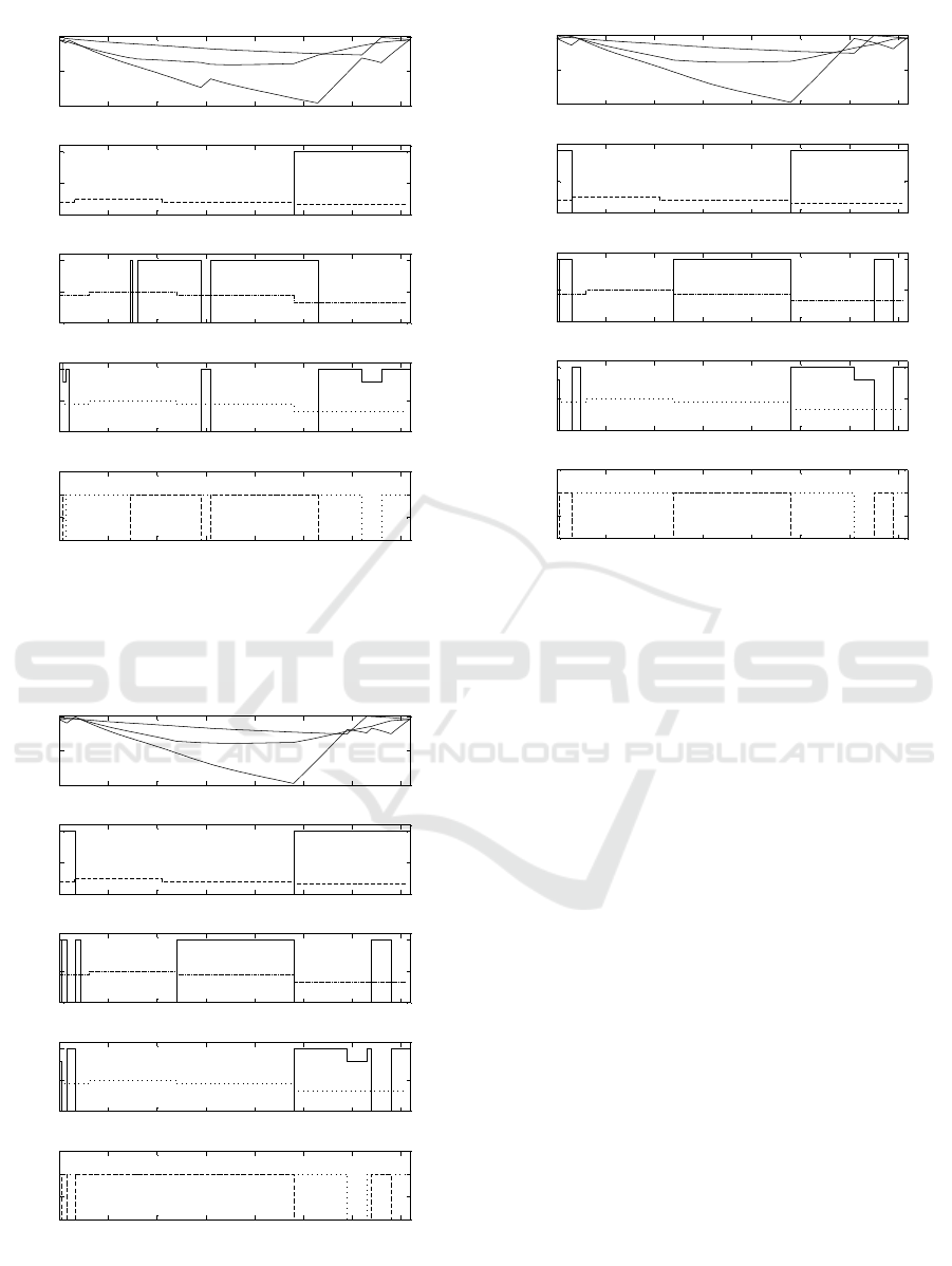
The result of the optimization with α = 0.05 is
shown in figure 4. The cost is similar, J = 17.23, but
there are only 15 pump and 8 valve commutations.
With α = 0.1, the result is a higher cost (J = 17.54),
but a really small number of commutations (10 pumps
and 6 valves).
The resulting number of commutations is highly
dependent on the weighting factor α. In order to fix a
desired value, the second approach consists of adding
as a constraint the number of commutations. The fig-
ure 5 shows the result of the optimization (38) when
the number of changes in δ is constraint to 20. The
cost index is J = 17.12 and the pump and valve com-
mutations 18 and 9, respectively.
Modelling and Optimization of the Operation of a Multiple Tank Water Pumping System
151
0 200 400 600 800 1000 1200 1400
0
50
100
Volumes (in %)
0 200 400 600 800 1000 1200 1400
0
100
200
Flow of pump 1
0 200 400 600 800 1000 1200 1400
0
50
100
Flow of pump 2
0 200 400 600 800 1000 1200 1400
0
50
100
Flow of pump 3
0 200 400 600 800 1000 1200 1400
0
0.5
1
1.5
Valves
Figure 2: Optimization result for period=5 minutes, L=4.
Volumes (in percentage), flow of pump 1, 2 and 3, and state
of valves.
The figure 6 shows the result of the optimization
when the number of changes in δ is constraint to 16.
The cost index is J = 17.1 and the pump and valve
commutations 15 and 9, respectively.
The results are similar to those obtained with the
previous approach (in terms of cost index), but the
constraint in the number of commutations is explicit.
7 CONCLUSIONS
In this paper we have studied the optimization of the
operation of a water supply pumping system by means
of standard solvers. The automatic operation of the
system tries to determine which valves and pumps
must be active at each instant of time in order to min-
imise the operation cost, taking into account the tar-
iff periods. The main constraints are the maximum
and minimum volumes of the tanks. A mathematical
model of the problem is proposed in order to formu-
late, in matrix form, the cost index and the constraints,
to be able to use standard solvers as Mosek or CBC. A
basic optimization problem is proposed, that only im-
poses the constraints of the finite volume of the tanks.
0 200 400 600 800 1000 1200 1400
0
50
100
Volumes (in %)
0 200 400 600 800 1000 1200 1400
0
100
200
Flow of pump 1
0 200 400 600 800 1000 1200 1400
0
50
100
Flow of pump 2
0 200 400 600 800 1000 1200 1400
0
50
100
Flow of pump 3
0 200 400 600 800 1000 1200 1400
0
0.5
1
1.5
Valves
Figure 3: Optimization result for period=5 minutes, L=4.
Volumes (in percentage), flow of pump 1, 2 and 3, and state
of valves. Cost index with number of changes, α = 0.02.
The result of this basic problem tends to produce a
large number of pump and valve commutations, that
is not adequate in practice. To solve this problem, two
alternatives are proposed: to include the number of
commutations in the cost index, and to add as a con-
straint the maximum number of commutations. Both
approaches lead to an adequate result, but the second
one is easier to use, as the number of commutations
can be fixed in an explicit way, while in the other ap-
proach the final number of commutations depends on
the weighting factor applied to the number of commu-
tations in the cost index. An example of a real water
supply system with 3 tanks, 3 pumps and 2 valves is
analysed to demonstrate the validity of the approach,
using Yalmip as parser and Mosek as solver. The ba-
sic optimization problem leads to a high number of
commutations, as expected. Including the number of
commutations in the cost index, or adding as a con-
straint the maximum number of commutations lead
to a slight increase in the cost while the number of
changes in the actuator states is maintained under a
reasonable level.
ICINCO 2017 - 14th International Conference on Informatics in Control, Automation and Robotics
152
0 200 400 600 800 1000 1200 1400
0
50
100
Volumes (in %)
0 200 400 600 800 1000 1200 1400
0
100
200
Flow of pump 1
0 200 400 600 800 1000 1200 1400
0
50
100
Flow of pump 2
0 200 400 600 800 1000 1200 1400
0
50
100
Flow of pump 3
0 200 400 600 800 1000 1200 1400
0
0.5
1
1.5
Valves
Figure 4: Optimization result for period=5 minutes, L=4.
Volumes (in percentage), flow of pump 1, 2 and 3, and state
of valves. Cost index with number of changes, α = 0.05.
0 200 400 600 800 1000 1200 1400
0
50
100
Volumes (in %)
0 200 400 600 800 1000 1200 1400
0
100
200
Flow of pump 1
0 200 400 600 800 1000 1200 1400
0
50
100
Flow of pump 2
0 200 400 600 800 1000 1200 1400
0
50
100
Flow of pump 3
0 200 400 600 800 1000 1200 1400
0
0.5
1
1.5
Valves
Figure 5: Optimization result for period=5 minutes, L=4.
Volumes (in percentage), flow of pump 1, 2 and 3, and state
of valves. Constraint in the number of changes, 20.
0 200 400 600 800 1000 1200 1400
0
50
100
Volumes (in %)
0 200 400 600 800 1000 1200 1400
0
100
200
Flow of pump 1
0 200 400 600 800 1000 1200 1400
0
50
100
Flow of pump 2
0 200 400 600 800 1000 1200 1400
0
50
100
Flow of pump 3
0 200 400 600 800 1000 1200 1400
0
0.5
1
1.5
Valves
Figure 6: Optimization result for period=5 minutes, L=4.
Volumes (in percentage), flow of pump 1, 2 and 3, and state
of valves. Constraint in the number of changes, 16.
ACKNOWLEDGEMENTS
This work has been supported by MICINN project
number TEC2015-69155-R from the Spanish govern-
ment.
REFERENCES
Bunn, S. and Reynolds, L. (2009). The energy-
efficiency benefits of pump scheduling optimiza-
tion for potable water supplies. IBM Jour-
nal of Research and Development, 53:5:1 – 5:13.
DOI:10.1147/JRD.2009.5429018.
Fang, H., Zhang, J., and liang Gao, J. (2010).
Optimal operation of multi-storage tank multi-
source system based on storage policy. Jour-
nal of Zhejiang University-SCIENCE A, 11:571–579.
DOI:10.1631/jzus.A0900784.
Martinez, F., Hernandez, V., Alonso, J., Rao, Z., and Alvisi,
S. (2007). Optimising the Operation of the Valencia
Water-Distribution Network. Journal of Hydroinfor-
matics, 9(1):6578.
Ormsbee, L., Lingireddy, S., and Chase, D. (2009). Optimal
Pump Scheduling For Water Distribution Systems. In
Proceedings of the 4
th
Multidisciplinary International
Conference on Scheduling : Theory and Applications
Modelling and Optimization of the Operation of a Multiple Tank Water Pumping System
153

(MISTA 2009), 10-12 August 2009, Dublin, Ireland,
pages 341–356.
Ormsbee, L. E. and Lansey, K. E. (1994). OPTIMAL CON-
TROL OF WATER SUPPLY PUMPING SYSTEMS.
Journal of Water Resources Planning and Manage-
ment, 120:237–252. ISSN:0733-9496/94/0002- 0237.
Pasha, M. F. K. and Lansey, K. (2009). Optimal Pump
Scheduling by Linear Programming. In Proceedings
of the 4
th
World Environmental and Water Resources
Congress 2009 May 17-21, 2009 — Kansas City, Mis-
souri, United States, pages 341–356.
Powell, R. S. and McCormick, G. (2004). Derivation of
NearOptimal Pump Schedules for Water Distribution
by Simulated Annealing. J. Operational Res. Soc,
55:728736.
Savic, D. A., Walters, G. A., and Schwab, M. (1997). Multi-
objective Genetic Algorithms for Pump Scheduling in
Water Supply. Springer-Verlag, London.
Sotelo, A., L
¨
ucken, C., and Bar
´
an, B. (2002). Multi-
objective Evolutionary Algorithms in Pump Schedul-
ing Optimization. In Proceedings of the Third Inter-
national Conference on Engineering Computational
Technology, Stirling, Scotland., page 175176.
Wegley, C., Eusuff, M., and Lansey, K. E. (2000). Deter-
mining Pump Operations Using Particle Swarm Op-
timization. In Proceedings of the Joint Conference
on Water Resources Engineering and Water Resources
Planning and Management, Minneapolis, 2000.
ICINCO 2017 - 14th International Conference on Informatics in Control, Automation and Robotics
154
