A Multi-objective Mathematical Model for Problems Optimization in

Multi-modal Transportation Network

Mouna Mnif

and Sadok Bouamamaa

1,2

ENSI, University of Manouba, COSMOS Laboratory, Tunisia

FCIT, University of Jeddah, K.S.A.

Keywords: Multimodal, Transportation Network, Optimization Problem, Mathematical Formulation, Multi-Objective

Optimization, Planning Problem.

Abstract: In order to reach a sustainable planning in a rather complicated transport system, it is of high interest to use

methods included in Operations Research areas. This study has been conducted to solve the transportation

network planning problems, in accordance with the optimization problem and multi-objective transport

network in multi-modal transportation. Firstly, we improve the implementation of the existing literature model

proposed in (Cai, Zhang, and Shao, 2010; Zhang and Peng, 2009) because after the conducted

experimentation, we show that there are two previously proposed constraints that make the solution

unrealizable for the transportation problem solving. Secondly, we develop the proposed multi-objective

programming model with linear constraints. Computational experiments are conducted to test the

effectiveness of the proposed model. The mathematical formulation is developed to contribute to success

solving the optimization problem, taking into account important aspects of the real system which were not

included in previous proposals in the literature, and review. Thus, it gives ample new research directions for

future studies.

1 INTRODUCTION

The multimodal transportation offers a full range of

transportation modes and routing options, allowing

them to coordinate supply, production, storage,

finance, and distribution functions to achieve the

most efficient relationships. The goal is to move from

the starting city to the destination city through other

intermediate cities, of which there are several routes

between two cities. In the multi-objective optimiza-

tion problem, the decision maker is charged by an

efficiency choice of existing routes in order to select

the best itinerary according to a compromise solution

between a set of objectives such as the minimization

of the transport cost and the duration of transport, the

maximization of service quality, etc.

The multimodal transportation network studies

were carried out by several problems such as

planning networks, shortest path, maritime or airline

with urban centers, freight transport, transmission

line, loading-unloading terminals, schedules, etc. The

focus of most widely research in the literature has

been based on planning network.

There are various measures to evaluate a multi-

modal path, for example, the travel cost, in-vehicle

time, waiting time, length, travel time, transfer time,

the number of transfers and so on. The optimization

and the operation research play an important role to

solve this problem. The main objective of this

problem is to determine the shortest and efficient way

of satisfying a set of objectives, and a set of

operational constraints according to customer

demands.

In general, the objective of a multimodal network

planning problem is to optimize reliable transport

chains for passenger or freight. The mathematical

formulation of the transit network design is usually

intractable by exact approaches. In (Wan and Lo,

2003) a MILP formulation that minimizes the

operating cost to a bus capacity constraint is

proposed. A characteristic of their formulation is that

it allows generating implicitly the structure of the

routes. However, this requires that a maximum

number of routes in the solution should be specified.

The objective minimizing the operating costs,

according to constraints within the system

considering the capacity and bounded exchange

action frequency.

The multimodal shortest path problem (M-SPP) is

concerned with finding a path from a specific origin

352

Mnif, M. and Bouamama, S.

A Multi-objective Mathematical Model for Problems Optimization in Multi-modal Transportation Network.

DOI: 10.5220/0006472603520358

In Proceedings of the 14th International Conference on Informatics in Control, Automation and Robotics (ICINCO 2017) - Volume 1, pages 352-358

ISBN: 978-989-758-263-9

to a particular destination in a given multimodal

network while minimizing total costs associated. The

complexity of finding multi-modal route is obviously

much higher than single modal one. The multi-criteria

multi-modal shortest path problem (MM-SPP) with

transfer delaying and arriving time-window

belongs to the set of problems, which are known as

NP-hard. In (Liu, Mu, and Yang, 2014; Liu, Yang,

Mu, Li, and Wu, 2013) the exact algorithms for

solving the MM-SPP to minimize the total travel time

have been suggested, in which the delaying time in

the transfer parking and the arriving at a time window

of destination are considered, as well as the total

travel cost.

Each case treated is defined by the specific

parameters at the problem type. Since, each variant

possesses its own characteristics, it requires a

different decision depending on the considered

context. These decisions are based on the

special characteristics of the transportation mode, and

on specific constraints of the treated problem. These

constraints are specified for each customer, vehicle,

mode, road or means of transport, as well as the type

of the problem.

Being based on the existing works of the literature

research, we have adopted a mathematical model,

while relying on the existent works with the

objectives, and constraints set to take into account the

recommendations made by experts according to the

hypotheses of our treated problem. This proposed

formulation will be cited and validated by tests, which

will be detailed in the rest of this paper.

The structure of our paper is organized as follows:

In section 2, we’ll present the construction model

with the proposed formulation in order to solve the

multi-objective and multimodal transportation

problem. Section 3 discusses our contribution and

motivation. Section 4 provides the proposed model by

some numerical experiments. Thereafter, in section 5

we will discuss a critical comment on our work by a

synthesis of the obtained results. Finally, section 6

concludes our work with a summary and proposes

some future research directions.

2 A MULTI-OBJECTIVE

MATHEMATICAL MODEL

The main objective of the multimodal network

problem is to determine a shortest and an optimal path

between a start point and an end point to according to

several criteria relating to the transportation mode or

the itinerary, etc., to satisfy a set of objectives that are

distinct to the treated case problem. In fact, a

multimodal problem requires the consideration of

multiple objectives and linked constraint of a

sequence of frequently used modes. For an optimal

choice of a transport mode or an itinerary by a

transport mode selected, the various criteria must be

taken into consideration, although these criteria are

conflicting.

The multi-objective optimization can be defined

as the problem that is finding a vector of decision

variables which satisfies all constraints and optimizes

a vector of objective functions. These functions from

a mathematical description of performance criteria

are usually in conflict with each other. In this paper,

we have treated a multi-objective optimization

problem. We consider the problem studied is to find

viable multimodal and multi-objective transport

processes, in order to minimize the total

transportation cost and the total time of the itinerary,

while respecting the arriving of goods at a customer

in the corresponding time window. First, we will

present and discuss the model of (Cai et al., 2010).

2.1 Model Assumptions and Code

Description

2.1.1 The Assumptions

Let us define the following assumptions as:

 Only one mode of transport and a path can be

chosen between two nodes to carry the goods.

 Transport costs are directly proportional to the

realization, namely, the choice of the quantity

and the unit transportation cost.

 The limited capacity constraint of each mode is

respected.

 If a vehicle arrives at the node before the start

date of his time window, he waits.

 Transshipment of goods can only happen once

more at each node.

2.1.2 The Sets and Settings

: The set of all nodes;

: The set of transport mode;

Q : The total quantity of goods;

P : The maximum transfers duration;

: The delay period at node i if delay occurred;

: The overhead expenses per hour if delay occurred

at node i;

A Multi-objective Mathematical Model for Problems Optimization in Multi-modal Transportation Network

353







: The transport cost of a unit quantity from node i

to node j, by using k

transport mode;







: The fee for transport mode changed from k to l

at the node i;







: The transport time from node i to node j, with

transport mode selected;





: The largest time windows of cargos arriving

from node i to node j;





: The shortest time windows of cargos arriving

from node i to node j;







: The transfer time from transport mode k to the

transport mode l at the node i;





: The vehicle capacity from the k

transportation

mode.





: The number of vehicles used by the k

transportation mode in order to transport the

whole quantity of the freights. With, 





 







 upward, that returning the smallest

integral value that is not less than 









2.1.3 The Decision Variables

The decision is related to the optimization process

which focuses on itinerary scheduling and the

decision of selecting each transportation mode of

corresponding transportation means. Thus, we need

to define the decision variables that explain the

variables associated with each considered parameter

of our treated problem. These decision variables are

used to express the constraints and optimization

criteria.



,



=

1 if the 



transport mode is selected from  to ,

0 otherwise





,

=

1 transport mode changed from  to  at ,

 ,

0 otherwise





=

1 if there is a delay at the node i

0 otherwise

2.1.4 The Formulation

The mathematical formulation is a determinant

step in the resolution step and the optimization step of

any problem. Indeed, it allows us to define and

characterize the sets, the parameters, the decision

variables, the optimization criteria and constraints

that will satisfy the specific decisions. The paper

presents an effective solution for determining the

shortest and efficient way of satisfying a certain set of

demands under several criteria and also a large set of

operational constraints. Our proposed formulation is

presented as follows:

Minimize

Ni Kk Kl

Ni Nj Kk

pfuycxSC .....



    



(1)

(2)



















































































     

     

0,...

Ni Kk Kl

Ni Nj Kk

Ni Nj

iji

Ni Kk Kl

Ni Nj Kk

puyaxttwMax

TWpuyaxtMax

(3)

Subject to

Njix







(4)

Njixx







(5)

Njiyxx

 ,.2

(6)

Niy

Kk Kl





 

(7)

NiPay

Ni Kk Kl





  

(8)

 

KlkNetjiyx

 ,,0,1,

(9)

The equations that describe this mathematical

formulation can be summarized as follows. Equation

(1) represents the first objective that seeks to

minimize the total cost of the multimodal network,

including the cost of the itinerary, transshipment cost

and overhead cost on delay. Equation (2) defines the

second objective, which seeks to minimize the total

duration of multimodal transportation, including the

period of the itinerary, changing period and delay

duration. Equation (3) expresses the third objective

that guaranteed the arriving at the destination in the

time window. Constraint (4) is specific to the

selection of transportation mode, that only one mode

of transport and one itinerary can be selected between

two nodes. If it is zero, it means that the i node is not

included in the transport. Equation (5) demonstrates

that in the itinerary the destination node is the start

node for the next itinerary. Constraint (6) shows that

Ni Kk Kl

Ni Nj Kk

puyaxt ...



    



ICINCO 2017 - 14th International Conference on Informatics in Control, Automation and Robotics

354

the selection of the route should be ensured by a

continuous itinerary. Equations (7) and (8) are

relative to the transshipment constraints. Constraint

(7) indicates that one change of transport mode can

happen once at each node. Constraint (8) represents

the maximum time to be respected by the total

transshipment time. The decision-making variables

taking the integer binary value are described by the

equation (9).

3 CONTRIBUTION AND

MOTIVATION

In this paper, we have proposed a multi-objective

mathematical program inspired from (Cai et al., 2010)

and (Zhang and Peng, 2009). The authors have

addressed the multi-modal transport problem with

full loads at time limit. The problem is defined by the

search of a multimodal path in order to reach the

destination through several cities, knowing that there

are several transport modes possible between any two

cities. Each itinerary is characterized by a transport

duration, a cost, and a transportation capacity

between two cities. In fact, the authors proposed a

combination model for multi-modal transport of full

loads with time window constraint. The considered

assumptions are: firstly only one mode of transport

can be selected between two cities and secondly, the

transport cost is linear with distance. The same model

defined in (Zhang and Peng, 2009)is presented in (Cai

et al., 2010). The distinction parameters between our

mathematical formulation and the one presented by

(Cai et al., 2010; Zhang and Peng, 2009) are

presented as follows:







: The transport distance from i to j with the 



transport mode selected, for j=i+1.

T: The time limit from start point to the end.

The distinction constraints that indicates:

 The cargos to be arriving in limited time.

 















  

















 

 That a number of cargos cannot exceed the

capacity of conveyance.







 

 The time-window between two nodes.

















 











 











Although, we describe the main improvements

made to the literature model. The first objective is to

minimize the total cost of transport. This cost is

measured by the sum of three terms. At the

transportation cost term, we replaced the distance

parameter by a measured relative to the goods

transported (the number of used units of transport),

according to experts of the domain. In our case, we

will ignore the setting of the distance since there is

only one path between two nodes made by the same

transport mode k. We also note that it is useless to

consider the distance parameter when calculating the

transportation cost. On the other hand, we show the

importance of considering the goods quantity and the

number of transport units used in measuring the

transportation cost.

The third objective is provided by the

transformation of the time window constraint 









































, to an

objective, which assured to the goods arrive at a well-

determined interval of time. The main reason for this

transformation is on the one hand, in order to give

more chance to find a compromise solution, which

can be eliminated when it is a constraint. In fact, the

given solution of a problem must satisfy all the

constraints while minimizing (or maximizing) one or

more objectives. On the other hand, when it is an

objective we can easily play on their weight or

priority relative to the other objective. Moreover, that

we can find a solution that is preferred according to a

customer that will be eliminated by this constraint.

Indeed, the requirements of customers are different.

In some cases, the customer prefers that the arrival of

their goods, regardless of the time of this

merchandise’s arrival.

Pointing out the limitation of the previous

formulation is indicated as follows. Taking into

account the constraints (4) and (5) on the model of

(Cai et al., 2010), the model resolution remains non-

feasible. With regard to the definition of constraint (4)

that express that cargos will be arriving in limited

time, we consider that it is useless to introduce the

first part of the expression proposed by the authors.

So, we limit the constraint to its second part.

The constraint (5) makes it a non-feasible problem,

because if we consider the example of a product

fertilizer with a quantity Q = 122 tons, we can't

transport all this quantity in a single vehicle. One

railroad car can carry 61 tons of fertilizers. Therefore,

two railroad cars are needed if railway transport is

selected. Each car can carry 35 tons per vehicle, if the

road transport is chosen, the total of 3.5 cars,

therefore, four cars are needed to transport all the

quantity. Each boat can carry 10 tons, if water

transport is selected, a total of 12.2 vessels, is taken

A Multi-objective Mathematical Model for Problems Optimization in Multi-modal Transportation Network

355

as 13 boats. So, the equation (5) with these data are

expressed as the following: by railroad

mode, by road transport mode and 

by maritime transport mode, which is an

impossible inequality. Consequently, this constraint

is missing a whole other decision variable. A new

parameter must be added a such as 



that is the

number of vehicle used by the transport mode k.

Therefore, this constraint becomes,











 . We consider the example test that is

provided by one compound fertilizer company

located in Linyi City.

The element of the first objective

 













depends only on to the parameter i,

so it must be replaced by















. In regards to

the element of the second objective

 









depends only on to the parameter i, so

it must be replaced by











. Therefore, the delay

in a city is compared to the desired arrival time.

When the index of the parameters are considered

according to i, j for j= i+ 1, then the passage is forced

by all the nodes according to an increasing order.

Therefore, the parameters should be defined by the

index i, j in order to guarantee that the choice of the

nodes and the order are provided by the model.

Based on the discussion of features, the

organization of multi-modal transportation modes,

and time-windows introduced, we defined a more

efficient model for multi-modal transport of full loads

with time-windows.

4 EXPERIMENTATION RESULTS

In this section, we present the obtained results that

show the capability of the proposed model for solving

a complex problem with multiple objectives (linear

and non-linear) simultaneously that proves their

efficiency in decision-making. This section is devoted

to presenting the computational experiments carried

out for assessing the performance of our

mathematical model. In fact, we implemented an

integer program for solving the multi-objective and

multimodal transportation networks planning models,

by using Concert Technology of CPLEX 12.4

Optimizers, with Microsoft Visual Studio 2010.

Computational experiments are conducted to test the

effectiveness of the proposed model.

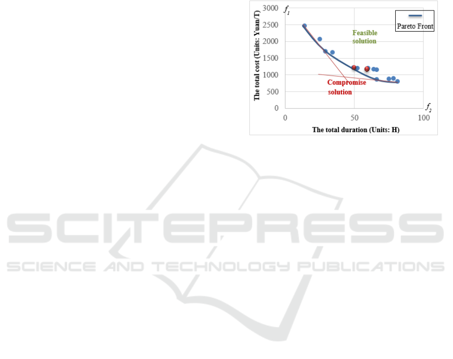
For a visual representation of the experimental

results, the reader is referred to Figure 1 as illustrated

below. The optimal solutions are represented by the

curve of the set of Pareto solution. The feasible

optimistic of the first objective vary between

max

2475.200 Yuan and

min

= 804.96 Yuan. The

optimistic solutions of the second objective vary

between

max

= 81H and

min

= 14 H. The optimistic

solutions of the third objective vary between

max

81H and

min

= 34 H. These solutions are obtained

by a set of tests sample generation.

Figure 1: Illustration of the Pareto optimality of a two

objectives minimization problem.

We observed that the third objective and the

second objective were synchronized objectives. But,

the two objectives are showing that they are clearly

contradictory with the first objective.

The overall measurement results are summarized

in Table 1 and 2 that are presented in the Appendix

section. The best solution that minimizes the first

objective gives a bad value for the second objective,

and vice versa. In this case, we must seek the solution

that satisfies the best compromise between these

objectives. This solution is presented in Figure 1 with

a red point, which is the closest value of the origin.

The Multiple Pareto optimal solutions based on five

distinct solutions found by the experimentations tests,

are represented by a blue curve in Figure 1. Hence, a

solution is called a Pareto optimal, if no feasible

vector exists which can decrease some criterion

without causing a simultaneous increase in at least

one criterion. In figure 1, a continuous line is used to

mark this boundary for a bi-objective minimization

problem in which, there is no single perfect solution

that minimizes both f

and f

. The aim is of

minimizing the compromise between the total cost

and the total duration for an itinerary of the

multimodal transportation network.

The set of all Pareto optimal solutions, called non-

dominated set or Pareto front, is located on the

boundary of the objective vector space (feasible

solution space) showing the tradeoff information

between the conflicting objectives. Instead, there are

compromises between optimal solutions such as the

solution presented by red. We can say that the

Compromise

solution

ICINCO 2017 - 14th International Conference on Informatics in Control, Automation and Robotics

356

solutions presented in the Pareto front are more

optimistic than the dominated solutions.

The various solutions which belong to the front of

Pareto are optimistic solutions. However, the

decision-maker is provided by the search of the best

compromise solution between the goals, which is

included on the Pareto Front. The CPLEX tool uses

the dynamic mixed-integer programming (MIP) as a

search method, the balance optimality, and feasibility

MIP emphasis. Indeed, the relaxation solution

obtained by a Branch and Cut algorithm through a

deterministic parallel mode, uses up to 4 threads.

The definition of Pareto optimality is similar to

that of efficiency, and a Pareto optimal point in the

criterion space is often considered the same as a non-

dominated point. Therefore, a solution is considered

as Pareto optimal, in a multi-objective minimization

problem, if there exists no other feasible solution

which would decrease some criteria without causing

a simultaneous increase in at least one criterion. This

set also called Pareto front helps the decision maker

to identify the best compromise solution by an

elimination of inferior ones. Then, the retained

solution as elite is the one which has the best

compromise between all the objectives.

5 DISCUSSION AND COMMENTS

According to the tests achieved for our work, giving

the priority to the first objective by minimizing the

total cost is much better than giving the executing

priority of the total duration which perfectly complies

with the third objective that respects the arriving at a

time window. Therefore, we note that the first

objective significantly improves the results as shown

in the Appendix.

For real case problems, the mathematical

formulation is not always reliable for a user, since we

cannot consider fixed rules for all possible

alternatives and treated cases associated with each

customer. According to the experts of a transit

company, the choice of transportation mode is

depends on the several factors, such as customer

requirements, the nature, and characteristics of the

goods, that can be a major condition for the selection

of the mode's problem. There are several features of

the goods, such as the expensive, bulky or perishable

goods, also the goods category or type such as

dangerous, fragile, light, stackable or non-stackable

goods, etc.

On the basis of the promising findings presented in

this paper, further research will be needed to solve

more optimization constraints. Artificial intelligence

approaches to the issue are still required. (Bouamama,

2010) proposed a multi-agent approach based on a

dynamic, distributed Practical Swarm Optimization

algorithm, which is proven to be useful for hard

optimization problems. (Mathlouthi and Bouamama,

2015) proposed two new approaches, a centralized

and distributed honey-bee optimization, enhanced by

a new parameter called local optimum detector. These

two approaches are applied to solve the maximal

constraint satisfaction problems.

6 CONCLUSIONS AND FUTURE

WORKS

This paper presents a new mathematical model in

order to solve multi-modal transport problems that

satisfy multiple objectives according to several

criteria. The proposed multi-objective model is

defined by three objectives, the minimization of the

total cost, and the total duration of an itinerary while

respecting the arriving of goods to a customer at the

time window.

In fact, the following conclusions can be drawn

as: Firstly, an improvement over the literature model

was achieved in order to find feasible solutions.

Secondly, a validation of our proposed model by

implementation. Thirdly, we summarized our work

by computation's test and experimentation results in

order to prove the efficiency of our model.

This paper presents a decision method based on a

mathematical model which plays a significant role in

resolving the transportation problem. Although there

has been a fruitful development of models and

solution techniques to solve this problem by a

relevant decision in transport networks, many future

pieces of research prospects are still missing, such as

the following:

 There are still opportunities for integrating

problems that can be solved separately, by using a

multi-criteria analysis approach.

 The development of robust, or dynamic

approaches used to solve a planning problem.

 The consideration of several types of

products, around on the corresponding product’s

cluster with the same characteristics, since the

choice of the transport mode depends on the

product volume and the value associated with

each product.

 The activation or cancellation of a goal according

to customer wishes by adding weights to each

objective, according to the client's need.

A Multi-objective Mathematical Model for Problems Optimization in Multi-modal Transportation Network

357

REFERENCES

Bouamama, S. (2010). A New Distributed Particle Swarm

Optimization. Knowledge-Based and Intelligent

Information and Engineering Systems, 312–321.

Cai, Y., Zhang, L., and Shao, L. (2010). Optimal multi-modal

transport model for full loads with time windows. 2010

International Conference on Logistics Systems and

Intelligent Management, ICLSIM 2010, 1, 147–151.

Liu, L., Mu, H., and Yang, J. (2014). Toward algorithms for

multi-modal shortest path problem and their extension in

urban transit network. Journal of Intelligent

Manufacturing, Springer S.

Liu, L., Yang, J., Mu, H., Li, X., and Wu, F. (2013). Exact

algorithms for multi-criteria multi-modal shortest path

with transfer delaying and arriving time-window in urban

transit network. Applied Mathematical Modelling, 38(9–

10), 2613–2629.

Mathlouthi, I., and Bouamama, S. (2015). A family of honey-

bee optimization algorithms for Max-CSPs.

International Journal of Knowledge-Based and

Intelligent Engineering Systems, 19(4), 215–224.

Wan, Q. K., and Lo, H. K. (2003). A Mixed Integer

Formulation for Multiple-Route Transit Network Design.

Journal of Mathematical Modelling and Algorithms,

2(4), 299–308.

Zhang, L., and Peng, Z. (2009). Optimization model for

multi-modal transport of full loads with time windows.

Proceedings - International Conference on Mana-

gement and Service Science, MASS 2009.

APPENDIX

Table 1: The experimentations tests in order of priority: objective 2 then objective 1.

Objective

IInf

Best integer

Cuts/Best Bound

ItCnt

Gap

Solutions

Z2*

integral

0.00%

Z1 if Z2*

2475.2

Z1 if Z2<=29

2003.40

integral

1701.57

0.00%

Z1 if Z2<=64

2725.69

---

904.3059

2725.69

904.3059

66.82%

1244.74

904.3059

27.35%

1158.2820

1244.74

Cuts:7

6.95%

1169.49

1158.2820

0.96%

Cutoff

1169.49

0.00%

Z1 if Z2<=75

1455.72

827.544

1455.72

827.544

43.15%

1168.19

827.544

29.16%

878.02

1168.19

Cuts:4

24.84%

884.62

878.02

0.75%

883.62

878.02

0.63%

Cutoff

883.62

0.00%

Table 2. The experimentations tests in order of priority: objective 1 then objective 2.

Objective

IInf

Best integer

Cuts/Best Bound

ItCnt

Gap

Solutions

Z1*

1153.89

integral

804.96

0.00%

Z2 if Z1*

Z2? if

Z1<=1170

75.0

51.6294

75.0

51.6294

31.16%

66.0

51.6294

21.77%

64.0

51.6294

19.33%

cutoff

64.0

0.00%

Z2? if

Z1<=1500

75.0

---

37.4761

75.0

37.4761

50.03%

49.0

37.4761

23.52%

46.0

37.4761

18.53%

39.2491

46.0

Cuts:5

14.68%

Cutoff

46.0

0.00%

ICINCO 2017 - 14th International Conference on Informatics in Control, Automation and Robotics

358