Using Polynomial Eigenvalue Problem Modeling to Improve Visual
Odometry for Autonomous Vehicles
Anderson Souza
1
, Leonardo Souto
2
, Fabio Fonseca de Oliveira
2
, Biswa Nath Datta
3
and Luiz M. G. Gonc¸alves
2
1
Department of Computing, University of the State of Rio Grande do Norte, Natal, RN, Brazil
2
Department of Computing Engineering and Automation, Federal University of the Rio Grande do Norte, Natal, RN, Brazil
3
Northern Illinois University, U.S.A.
Keywords:
Visual Odometry, Polynomial Eigenvalue Problem, Motion Estimation.
Abstract:
Visual Odometry (VO) is the process of calculating the motion of an agent (such as, robot and vehicle), using
images captured by a single or multiple cameras embedded to it. VO is an important process to supplement
autonomous navigation systems, since VO can provide accurate trajectory estimates. However, algorithms
of VO work with several steps of hard numerical computation which generate numerical errors and demand
considerable processing time. In this paper, we propose the use of a mathematical framework for monocular
VO process based on Polynomial Eigenvalue Problem (PEP) modeling in order to achieve both more accurate
motion estimation and to decrease the processing time of the VO process. Some previous experiments are
shown in order to validate the proposed computation accuracy.
1 INTRODUCTION
Nowadays, it is common to see autonomous agents
such as robot and vehicle to perform different tasks.
It is possible to find out these devices transport-
ing materials in factories, transporting people in ur-
ban zone, monitoring environments, exploring areas,
in surveillance, among other applications (Siegwart
et al., 2011).
Autonomous agents must be able to collect infor-
mation about their environment; considering this in-
formation, they must make some decision in order to
decide how to proceed, facing what exists in the envi-
ronment; and have to actuate in order to perform the
previous decision, towards completing their mission
(Murphy, 2000). An important condition for agents
achieving these abilities is that they must be equipped
with sensors, which provide them useful information
of their environment. In this way, a robot or a vehi-
cle can interact coherently with its environment and
objects, leading with unexpected situations like, dy-
namic obstacles (Souza and Gonc¸alves, 2015).
Cameras are widely used as visual sensor systems
for autonomous robots and vehicles. These systems
can be composed by a single or multiples cameras and
a mechanism for computing cameras data, which
allows the extraction of useful information from raw
data (Ma et al., 2004). With a visual sensor sys-
tem it is possible to infer a plenty of information
such as colors, textures, geometric structures, object
recognition, among others. Furthermore, it is feasible
to estimate relative or absolute motion, from images
captured from different positions, Visual Odometry -
VO. This is an important operation to supplement au-
tonomous navigation systems, since VO can provide
accurate trajectory estimates (Scaramuzza and Fraun-
dorfer, 2011).
However, processing raw data captured by cam-
eras in order to extract useful information, goes
through several numerical computation steps, which
produce numerical errors (overflow and underflow),
round-off errors and error bound. Moreover, these
computations consume significant processing time
demanded by algebraic calculations with vectors and
matrices (Datta, 2010). Both aspects (errors effects
and time processing) need to be minimized so that
they do not cause damages to the autonomous navi-
gation process by misinterpreted information (due to
miscalculations), or through decisions not taken in
time.
In this context, this paper proposes the use of a
mathematical framework for monocular VO process
502
Souza, A., Souto, L., Oliveira, F., Datta, B. and Gonçalves, L.
Using Polynomial Eigenvalue Problem Modeling to Improve Visual Odometry for Autonomous Vehicles.
DOI: 10.5220/0006478005020507
In Proceedings of the 14th International Conference on Informatics in Control, Automation and Robotics (ICINCO 2017) - Volume 2, pages 502-507
ISBN: Not Available
Copyright © 2017 by SCITEPRESS – Science and Technology Publications, Lda. All rights reserved

based on Polynomial Eigenvalue Problem (PEP)
modeling in order to achieve both more accurate mo-
tion estimation and decreasing the processing time of
the VO process. In this way, the VO process can be
analyzed as a minimum problem and it can be solved
by using polynomial equations systems (Kukelova
et al., 2012). In order to validate the proposed mod-
eling in terms of accuracy, preliminary experiments
with real data are presented.
This paper is organized as follow: section 2 intro-
duces the Visual Odometry problem for a monocular
vision system. Section 3 provides the formulation of
PEP. Section 4 shows the Visual Odometry modeled
as a PEP. Section 5 presents some preliminary experi-
ments. Finally, some considerations and future works
are presented in section 6.
2 MONOCULAR VISUAL
ODOMETRY
Localization is a fundamental point in autonomous
navigation. An autonomous robot or vehicle needs to
be able to estimate its position and orientation relative
to its environment. Visual Odometry - VO is process
that can provide accurate trajectory estimates. VO op-
erates by incrementally estimating the pose (position
and orientation) of an agent through examination of
the changes that motion induces on images of its on-
board cameras (Scaramuzza and Fraundorfer, 2011).
VO process can be performed by multiples cam-
eras or a single camera, which is named monocular
VO. In this case, motion and 3D structures are com-
puted from 2D images data. Feature-based methods
is one of the main approaches for estimating poses in
monocular VO. These methods are based on salient
and repeatable features that are tracked over consecu-
tive frames (Scaramuzza and Fraundorfer, 2011).
VO computes the camera path incrementally, pose
after pose (for simplicity, it is common to assume
that the camera coordinate frame to be the agent
coordinate frame). In order to do this, the main
point is to compute the relative transformation T
k
∈
R
4×4
, (k = 1, ...,n), from consecutive images (I
k−1
,I
k
)
taken at times k − 1 and k and then, concatenate the
transformation to recover the full trajectory C
0:n
=
{C
0
,C
1
,...,C
n
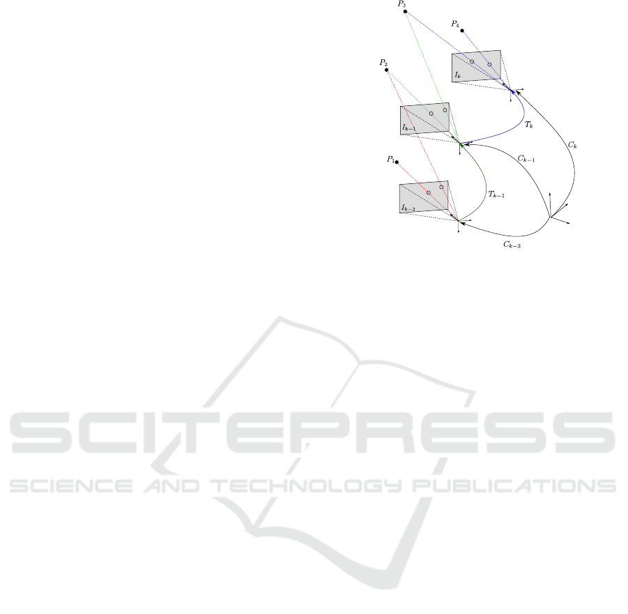
}. Figure 1 illustrates this process. T
k
is
often called rigid body motion and can be described
as:
T
k
=

R
k
t
k
0 1

(1)
R
k
∈ SO(3) and t
k
∈ R
3×1
are the rotation ma-
Figure 1: The relative motion T
k
is calculated from features
(projections of P
2
and P
3
) and after, it is concatenated to
obtain the absolute pose C
k
.
trix and the translation vector, respectively. These pa-
rameters can be computed by estimating the essential
matrix E, which describes the geometric relation be-
tween two images I
k
and I
k−1
of a calibrated camera,
up to a scale factor, as shown in Equation (2).
E
k
≃
ˆ
t
k
R
k
(2)
where t
k
= [t
x
,t
y
,t
z
]
T
and
ˆ
t
k
=



0 −t
z
t
y
t
z
0 −t
x
−t
y
t
x
0



(3)
It is known that in the case of fully calibrated
cameras points q and q
′
(from I
k−1
and I
k
, respec-
tively), which are projections of 3D points P (Figure
1), are geometrically constrained by the epipolar ge-
ometry constraint (Kukelova et al., 2012), formulated
by Equation (4).
q
′
E
k
q = 0 (4)
where the essential matrix E
k
is a 3× 3 rank-2 matrix
with two equal singular values. These constraints can
be presented in an other way, as shown in Equations
(5) and (6).
det(E
k
) = 0 (5)
2E
k
E
T
k
E
k
− trace(E
k
E
T
k
)E
k
= 0 (6)
Five-points algorithm proposed by Nister (Nis-
ter, 2004) and eight-points algorithm proposed by
Longuet-Higgins (Longuet-Higgins, 1981) are the
most popular approaches for computing the essential
matrix E
k
and, recovering R
k
and t
k
. In this paper,
Using Polynomial Eigenvalue Problem Modeling to Improve Visual Odometry for Autonomous Vehicles
503

we focus on the polynomial eigenvaluesolution to the
five-points algorithm for estimating E
k
.
Usually, after getting a possible result of E
k
, a
nonlinear optimization step is performed in order to
obtain more accurate estimate of T
k
.
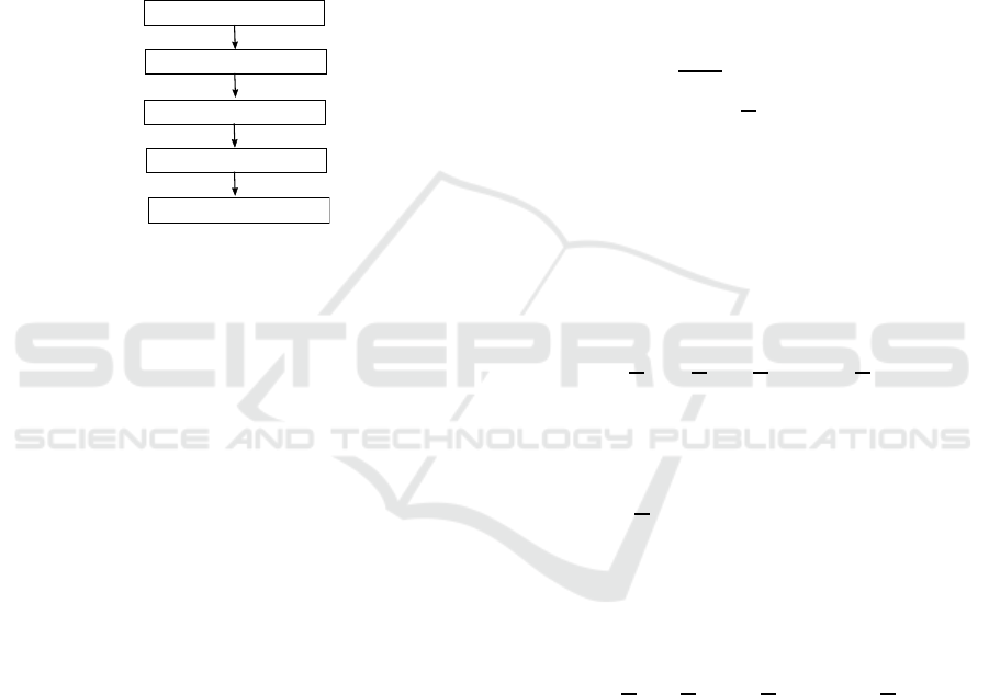
The VO process is often summarized into some
steps as shown in Figure 2. Further information about
VO can be found in (Scaramuzza and Fraundorfer,
2011) and (Scaramuzza and Fraundorfer, 2012), in-
cluding mathematical formulation of VO problem,
feature selection methods, matching, robustness and
optimization approaches and applications.
Image Sequence
Feature Matching
Feature Detection
Motion Estimation
Local Optimization
Figure 2: Steps of the monocular feature-based VO process.
3 POLYNOMIAL EIGENVALUE
PROBLEMS
Following definitions and formulation presented in
(Kukelova et al., 2012) and (Betcke et al., 2013),
polynomial eigenvalue problems (PEP) are problems
of the form presented by Equation (7), in which the
main purpose is to find scalars λ and nonzero vectors
v that satisfy the equation.
C(λ)v = 0 (7)
In this equation, v is vector of monomials in all
variables except for λ, andC(λ) is a n×n matrix poly-
nomial in variable λ defined as
C(λ) ≡ λ
l
C
l
+ λ
l−1
C
l−1
+ ... + λC
1
+C
0
, (8)
with n× n coefficient matrices C
j
.
A polynomial eigenvalue problem (PEP) can be
also represented as a standard generalized eigenvalue
problem (GEP) with the form
Ax = λBy (9)
Consider the following polynomial equation
(PEP),
(λ
l
C
l
+ λ
l−1
C
l−1
+ ... + λC
1
+C
0
)v = 0 (10)
It can be transformed to a GEP with,
A =





0 I 0 ... 0
0 0 I ... 0
... ... ... ... ...
−C
0
−C
1
−C
2
... −C
l−1





, (11)
B =





I
...
I
C
l





,y =





v
λv
...
λ
l−1
v





IfC
l
is nonsingular and well conditioned, it is pos-
sible consider a monic matrix polynomial,
C(λ) = C
−1
l
C(λ) (12)
with coefficient matrices
C
i
= C
−1
l
C
i
, i = 0,... ,l − 1.
Thus, Equation (10) can be transformed to
Ay = λy, (13)
where
A =





0 I 0 ... 0
0 0 I ... 0
... ... ... ... ...
−
C
0
−C
1
−C
2
... −C
l−1





(14)
In some cases, matrixC
l
is singular, in contrast the
matrix C
0
is regular and well conditioned. Thus, ei-
ther the described method which transforms PEP (10)
to the GEP (11) or the transformation β = 1/λ can be
used. Then,
C
i
= C
−1
0
C
i
, i = 1...l and matrix A gets
the form
A =





0 I 0 ... 0
0 0 I ... 0
... ... ... ... ...
−
C
l
−C
l−1
−C
l−2
... −C
1





(15)
The transformation β = 1/λ reduces the problem
to finding eigenvalues of the matrix (Kukelova et al.,
2012). There are many efficient numerical algorithms
for solving this GEP, like the QZ algorithm (Datta,
2010).
4 PEP SOLUTION FOR VISUAL
ODOMETRY
As mentioned before, five-points algorithm (Nister,
2004) is one of the most common approach for the
ICINCO 2017 - 14th International Conference on Informatics in Control, Automation and Robotics
504

Visual Odometry problem. It has become the stan-
dard for monocular motion estimation in the presence
of outliers (Scaramuzza and Fraundorfer, 2011).
Kukelova and colleagues (Kukelova et al., 2012)
propose a solution based on PEP for relative pose
problems using part of the five-points algorithm, and
their formulation is used in this paper for the monoc-
ular visual odometry problem.
The five-points algorithm requires m ≥ 5, with m
been the number of points with correspondence in
two consecutive images. Each of the point correspon-
dences gives rise to a constraint of the form (4). This
constraint can also be written as
˜q
T
˜
E = 0 (16)
where
˜q ≡ [q
1
q
′
1
,q
2
q
′
1
,q
3
q
′
1
,q
1
q
′
2
,q
2
q
′
2
,q
3
q
′
2
,q
1
q
′
3
,q
2
q
′
3
,q
3
q
′
3
]
T
˜
E = [e
11
,e
12
,e
13
,e
21
,e
22
,e
23
,e
31
,e
32
,e
33
]
T
By stacking the vectors ˜q
T
for five points, a 5×9 ma-
trix is obtained. The null space of this matrix gener-
ates four vectors
˜
E
1
,
˜
E
2
,
˜
E
3
and
˜
E
4
that span it. They
can be found by SVD or QR decomposition. With
these vectors one can create four correspondent 3× 3
matrices, E
1
, E
2
, E
3
and E
4
. The essential matrix E
can be constructed as a linear combination of these
matrices, as shown by Equation (17).
E = xE
1
+ yE
2
+ zE
3
+ E
4
(17)
for some scalars x, y and z. Now, it is used the rank
constraint (5) and the trace constraint (6) to build 10
third-order polynomial equations in three unknowns
and 20 monomials. These equations can be written
as:
MX = 0 (18)
where M is a 10 coefficient matrix reduced by
Gauss-Jordan elimination and X = [x
3
,yx
2
,y
2
x,
y
3
,zx
2
,zyx, zy
2
,z
2
x,z
2
y,z
3
,x
2
,yx, y
2
,zx,zy,z
2
,x, y, z,1]
T
is the vector of all monomials. There are all mono-
mials in three unknowns up to degree three. At this
point, Equation (10) must be recovered, and taking
λ = z, Equation (17) can be written as
(z
3
C
3
+ z
2
C
2
+ zC
1
+C
0
)v = 0 (19)
where v vector of monomials, v =
[x
3
,x
2
y,xy
2
,y
3
,x
2
,xy,y
2
,x, y, 1]
T
and C
3
, C
2
, C
1
,
and C
0
are 10× 10 coefficient matrices given by:
C
3
= [0 0 0 0 0 0 0 0 0 m
10
],
C
2
= [0 0 0 0 0 0 0 m
8
m
9
m
16
],
C
1
= [0 0 0 0 m
5
m
6
m
7
m
14
m
15
m
19
],
C
0
= [m
1
m
2
m
3
m
4
m
11
m
12
m
13
m
17
m
18
m
20
].
where m
j
is the jth column from M.
The rank of the matrix C
3
is one and the matrix
C
0
is regular. Then, the transformation β = 1/z, pre-
sented in section 3, is possible and it reduces the cubic
PEP (19) to the problem of finding the eigenvalues of
the 30× 30 matrix A, Equation (20).
A =



0 I 0
0 0 I
−c
−1
0
C
3
−C
−1
0
C
2
−C
−1
0
C
1



(20)
From (20) 30 eigenvalues can be obtained, solu-
tions for β = 1/z, and 30 corresponding eigenvectors
v from which the solutions for x and y is extracted.
Hence, the essential matrix can be estimated by Equa-
tion (17).
After that, R and t are recovered. Let the sin-
gular value decomposition of the essential matrix be
E ∼ Udiag(1, 1, 0)V
T
, where U and V are cho-
sen such that det(U) > 0 and det(V) > 0. Then,
t
u
≡ [u
13
,u
23
,u
33
]
T
and R is equal to R
a
≡ UDV
T
or
R
b
≡ UD
T
V
T
(Nister, 2004).
Any combination of R and t satisfies the epipolar
constraint (16). Therefore, four possible solutions for
the transformation T
k
arise:
T
a
k
=

R
a
t
u
0 1

,T
b
k
=

R
a
−t
u
0 1

T
c
k
=

R
b
t
u
0 1

,T
d
k
=

R
b
−t
u
0 1

The true configuration is found by triangulating
one point of the images for one of each possible solu-
tion and verifying if its coordinate in the space yield a
position in front of the camera. Further details of the
triangulation step can be found in (Nister, 2004).
5 PRELIMINARY EXPERIMENTS
This section shows some preliminary steps imple-
mented to validate the proposed framework of VO
computation in terms of accuracy.
5.1 Image Capturing and Feature
Detection
For this first experiments, the KITTI dataset (Geiger
et al., 2012) was used to provide the sequence of im-
ages and the ground truth of a real vehicle. The FAST
(Features from Accelerated Segment Test) (Rosten
Using Polynomial Eigenvalue Problem Modeling to Improve Visual Odometry for Autonomous Vehicles
505

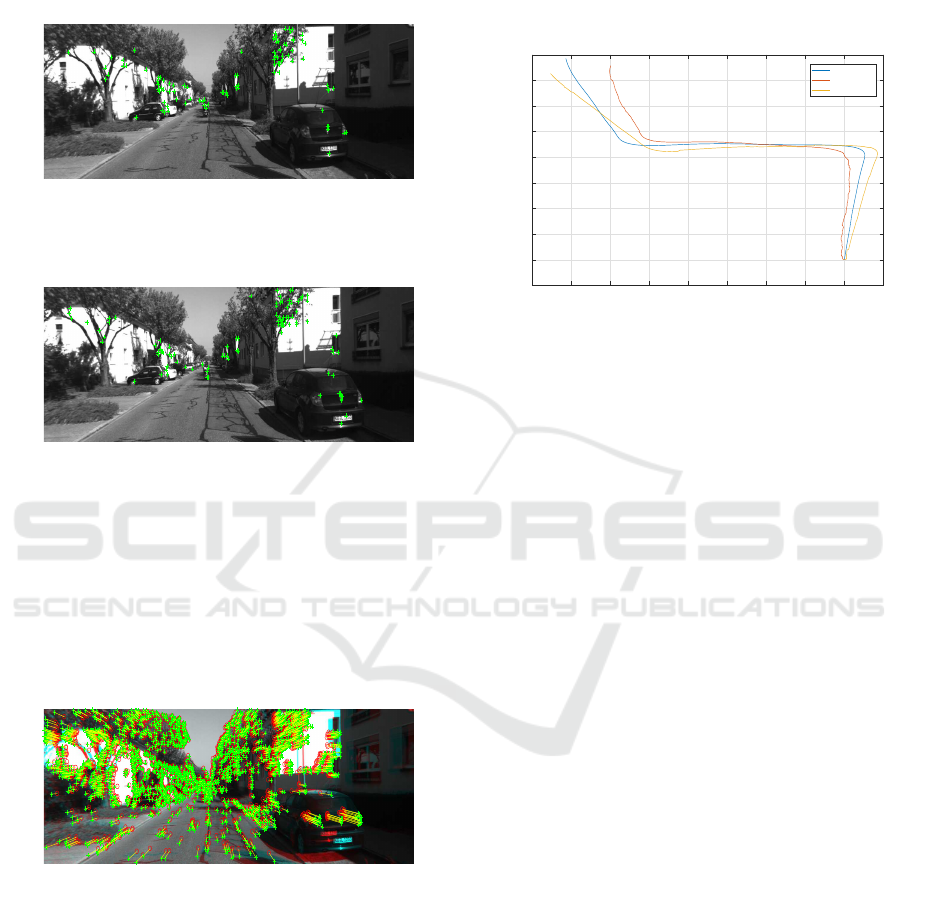
et al., 2010) algorithm was applied on the images in
order to identifies corners in consecutive images.
Figures 3 and 4 show features detected in consec-
utive images from the KITTI dataset.
Figure 3: Corners detected fromthe first image taken at time
k− 1.
Figure 4: Corners detected from the second image taken at
time k.
5.2 Feature Matching
In this step was used the FLANN (Fast Library for
Approximate Nearest Neighbors) algorithm (Muja
and Lowe, 2009), which matches the detected cor-
ners. Figure 5 illustrates a matching sampling.
Figure 5: Matching example.
5.3 VO Experiment
An experiment was performed in order to compare the
traditional implementation of VO using the Nister’s
five-point algorithm (Nister, 2004) and the implemen-
tation based on PEP with the modeling proposed by
Kukelova and colleagues (Kukelova et al., 2012).
Figure 6 presents a monocular VO process per-
formed with a set of 400 images from KITTI dataset.
The figure shows that the PEP solution is closer to
the ground truth line, indicating that the PEP solution
is more accurate than the VO based on the Nister’s
five-point algorithm. This happened due to numerical
robustness yield by the PEP solution.
-80 -70 -60 -50 -40 -30 -20 -10 0 10
X coordinates [m]
-20
0
20
40
60
80
100
120
140
160
Y coordinates [m]
Ground truth
Nister's 5pts
PEP Vo
Figure 6: Comparative experiment with VO based on Nis-
ter’s five-points algorithm and PEP solution.
6 CONCLUSION
This paper presented Monocular Visual Odometry
(VO) computing solution based on Polynomial Eigen-
value Problem for the five-points algorithm. VO
algorithms work with several step of hard numer-
ical computation which generate numerical errors
like overflow, underflow, round-off errors and error
bound, and demand considerable processing time.
VO process based on Polynomial Eigenvalue Prob-
lem (PEP) achieved more accurate motion estimation,
since PEP solutions achieve more numerical robust-
ness, as shown in a previous experiment.
As future works, the proposed method will be im-
proved with more robust optimization step and new
analysis comparing accuracy and processing will be
performed.
The final idea is to apply the VO algorithm in a
quadcopter vehicle in order to supply it with a esti-
mation of its trajectory.
ACKNOWLEDGEMENTS
We would like to thank CAPES for the financial sup-
port.
ICINCO 2017 - 14th International Conference on Informatics in Control, Automation and Robotics
506

REFERENCES
Betcke, T., Higham, N. J., Mehrmann, V., Schr¨oder, C., and
Tisseur, F. (2013). Nlevp: A collection of nonlinear
eigenvalue problems. ACM Transactions on Mathe-
matical Software (TOMS), 39(2).
Datta, B. (2010). Numerical Linear Algebra and Applica-
tions. SIAM Publishing, second edition edition.
Geiger, A., Lenz, P., and Urtasun, R. (2012). Are we ready
for autonomous driving? the kitti vision benchmark
suite. In Conference on Computer Vision and Pattern
Recognition (CVPR).
Kukelova, Z., Bujnak, M., and Pajdla, T. (2012). Poly-
nomial eigenvalue solutions to minimal problems in
computer vision. IEEE Transaction on Pattern Analy-
sis and Machine Intelligence, 34(7):1381–1391.
Longuet-Higgins, H. (1981). A computer algorithm for re-
constructing a scene from two projections. Nature,
293(10):133–135.
Ma, Y., Soatto, S., Kosecka, J., and Sastry, S. (2004). An
Invitation to 3-D Vision: From Images to Geometric
Models. Springer.
Muja, M. and Lowe, D. (2009). Fast approximate nearest
neighbors with automatic algorithm configuration. In
International Conference on Computer Vision Theory
and Application.
Murphy, R. (2000). Introduction to AI Robotics. MIT Press.
Nister, D. (2004). An efficient solution to the five-point
relative pose. IEEE Transaction on Pattern Analysis
and Machine Intelligence, 26(6):756–770.
Rosten, E., Porter, R., and Drummond, T. (2010). Faster
and better: a machine learning approach to corner de-
tection. IEEE Trans. Pattern Analysis and Machine
Intelligence, 32.
Scaramuzza, D. and Fraundorfer, F. (2011). Visual odome-
try - part i: The first 30 years and fundamentals. IEEE
Robotics and Automation Magazine, 18(4):1–18.
Scaramuzza, D. and Fraundorfer, F. (2012). Visual odom-
etry - part ii: Matching, robustness, optimization, and
applications. IEEE Robotics and Automation Maga-
zine, 19(2):78–90.
Siegwart, R., Nourbakhsh, I., and Scaramuzza, D. (2011).
Introduction to Autonomous Mobile Robots. MIT
Press, 2nd edition.
Souza, A. and Gonc¸alves, L. M. G. (2015). Occupancy-
elevation grid: An alternative approach for robotic
mapping and navigation. Robotica, Cambridge Uni-
versity Press, pages 1–18.
Using Polynomial Eigenvalue Problem Modeling to Improve Visual Odometry for Autonomous Vehicles
507