
An Information Theory Subspace Analysis Approach with Application to
Anomaly Detection Ensembles
Marcelo Bacher, Irad Ben-Gal and Erez Shmueli
Department of Industrial Engineering, Tel-Aviv University, Tel-Aviv, Israel
Keywords:
Subspace Analysis, Rokhlin, Ensemble, Anomaly Detection.
Abstract:
Identifying anomalies in multi-dimensional datasets is an important task in many real-world applications. A
special case arises when anomalies are occluded in a small set of attributes (i.e., subspaces) of the data and
not necessarily over the entire data space. In this paper, we propose a new subspace analysis approach named
Agglomerative Attribute Grouping (AAG) that aims to address this challenge by searching for subspaces that
comprise highly correlative attributes. Such correlations among attributes represent a systematic interaction
among the attributes that can better reflect the behavior of normal observations and hence can be used to im-
prove the identification of future abnormal data samples. AAG relies on a novel multi-attribute metric derived
from information theory measures of partitions to evaluate the ”information distance” between groups of data
attributes. The empirical evaluation demonstrates that AAG outperforms state-of-the-art subspace analysis
methods, when they are used in anomaly detection ensembles, both in cases where anomalies are occluded
in relatively small subsets of the available attributes and in cases where anomalies represent a new class (i.e.,
novelties). Finally, and in contrast to existing methods, AAG does not require any tuning of parameters.
1 INTRODUCTION
Anomaly detection refers to the problem of find-
ing patterns in data that do not conform to an ex-
pected norm behavior. These non-conforming pat-
terns are often referred to as anomalies, outliers, or
unexpected observations, depending on the applica-
tion domains (Chandola et al., 2007). Algorithms for
detecting anomalies are extensively used in a wide va-
riety of application domains such as machinery mon-
itoring (Ge and Song, 2013), sensor networks, (Ba-
jovic et al., 2011), and intrusion detection in data net-
works (Jyothsna et al., 2011).
In a typical anomaly detection setting, only nor-
mal or expected observations are available, and con-
sequently, some assumptions regarding the distribu-
tion of anomalies must be made to discriminate nor-
mal from anomalous observations (Steinwart et al.,
2006). Traditional approaches for anomaly detec-
tion (see, e.g., (Aggarwal, 2015)) often assume that
anomalies occur sporadically and are well separated
from the normal data observations, or that anoma-
lies are uniformly distributed around the normal ob-
servations. However, in complex environments, such
assumptions may not hold. For instance, if during
the analysis of the multi-attribute data generated in
a complex system only a few sensors fail to function
normally, only some of the data attributes will be af-
fected. From a data analysis perspective, these mal-
functions can be seen as data samples corrupted by
noise over a subset of data attributes. Consequently,
anomalies in the generated data might only be no-
ticeable in some projections of the data into a lower-
dimensional space, called a subspace, and not in the
entire data space. Also, consider a case where anoma-
lies represent a new, previously unknown, class of
data observations, commonly called novelties (Chan-
dola et al., 2007). Similarly to the malfunctions ex-
ample above, deviations from the original data obser-
vations might only be evident along a subset of at-
tributes. Yet, these attributes will often be correlated
in some sense, and therefore cannot be treated as cor-
rupted by noise.
Based on this observation, ensembles were pro-
posed as a novel paradigm in the anomaly detec-
tion field (Aggarwal and Yu, 2001). Ensembles for
anomaly detection typically follow three general steps
(Lazarevic and Kumar, 2005). First, a set of sub-
spaces is generated (e.g., by randomly selecting sub-
sets of attributes). This step is commonly referred to
as subspace analysis. Then, classical anomaly detec-
tion algorithms are applied on each subspace to com-
Bacher M., Ben-Gal I. and Shmueli E.
An Information Theory Subspace Analysis Approach with Application to Anomaly Detection Ensembles.
DOI: 10.5220/0006479000270039
In Proceedings of the 9th International Joint Conference on Knowledge Discovery, Knowledge Engineering and Knowledge Management (KDIR 2017), pages 27-39
ISBN: 978-989-758-271-4
Copyright
c
2017 by SCITEPRESS – Science and Technology Publications, Lda. All rights reserved

pute local anomaly scores. Finally, these local scores
are aggregated to derive a global anomaly score (e.g.,
using voting). Here, we focus on the subspace anal-
ysis stage, which aims at to finding a representative
set of subspaces, among a very large number of pos-
sible subspaces, such that anomalies can be identified
effectively and efficiently.
Several methods for subspace analysis have been
proposed in the literature. These methods can be clas-
sified into three broad approaches. The most basic
one is based on a random selection of attributes (see,
e.g., (Lazarevic and Kumar, 2005)). Other methods
search for subspaces by giving anomalous grades to
data samples, thus coupling the search for meaningful
subspaces with the anomaly detection algorithm (see,
e.g., (M
¨
uller et al., 2010)). Recent methods search
for subspaces that comprising of highly correlative at-
tributes (e.g., (Nguyen et al., 2013a)).
However, all of the above methods suffer from
one or more of the following limitations: (i) Some
attributes might not be included in the generated set
of subspaces. This might impact the effectiveness
of the ensemble since anomalies might occur any-
where in the data space. (ii) The set of generated sub-
spaces might contain thousands of subspaces which
may make the training and operation phases of the
ensemble computationally prohibitive. (iii) They re-
quire, prior to their execution, the tuning of param-
eters such as the number of subspaces, the maxi-
mal size of each subspace, the number of clusters or
information-theory thresholds.
To address the challenges mentioned above, we
developed the Agglomerative Attribute Grouping
method (AAG) for subspace analysis. Motivated by
previous works, AAG searches for subspaces that
comprise of highly correlative attributes. As a gen-
eral measure for attribute association, AAG applies a
metric derived from concepts of information-theory
measures of partitions (see e.g. (Simovici, 2007)). In
particular, AAG makes use of the Rokhlin distance
(Rokhlin, 1967) to evaluate the smallest distance be-
tween subspaces in the case of two attributes, and a
multi-attribute distance, which is proposed here, for
cases where more than two attributes are involved.
Then, AAG applies a variation of the well-known ag-
glomerative clustering algorithm where subspaces are
greedily searched by minimizing the multi-attribute
distance. We also propose a pruning mechanism that
aims at improving the convergence time of the pro-
posed algorithm while limiting the size of the sub-
spaces.
Several important characteristics differentiate
AAG from existing state-of-the-art approaches. First,
due to the agglomerative approach in the subspace
search, none of the data attributes is are discarded,
and attributes are combined in an effective way man-
ner to generate the set of subspaces. Second, the set
of subspaces that AAG generates is relatively “com-
pact” in comparison to existing methods for two main
reasons: the use of the agglomerative approach re-
sults in a relatively small number of subspaces, and
the pruning mechanism results in a relatively small
number of attributes in each subspace. Finally, as a
result of combining the agglomerative approach with
the minimization of the suggested distance measure,
AAG does not require any tuning of parameters.
To evaluate the proposed AAG method, we con-
ducted extensive experiments on publicly available
datasets, while using seven different classical and
state-of-the-art subspace analysis methods as bench-
marks. The results of our evaluation shows that an
AAG-based ensemble for anomaly detection: (i) out-
performs classical and state-of-the-art subspace anal-
ysis methods when used in anomaly detection ensem-
bles, in cases where anomalies are occluded in small
subsets of the data attributes, as well as in cases where
anomalies represent a new class (i.e., novelties); and
(ii) generates fewer subspaces with a smaller (on aver-
age) number of attributes, in comparison to the bench-
mark approaches, thus, resulting in a faster training
time for the anomaly detection ensemble.
The rest of the paper is organized as follows: Sec-
tion 2 discusses the background and related work.
Section 3 provides a review of relevant theoretical el-
ements whereas in Section 4 we detail the proposed
approach. Section 5 describes the experimental eval-
uation of our technique as well as provides a discus-
sion on the obtained results. Finally, we conclude in
section 6 and suggest future research directions.
2 BACKGROUND
In Machine Learning applications, anomaly detection
methods aim to detect data observations that consid-
erably deviate from normal data observations (Aggar-
wal, 2015). Well-documented surveys on anomaly
detection techniques are (Markou and Singh, 2003;
Chandola et al., 2007; Maimon and Rockach, 2005;
Pimentel et al., 2014) and (Aggarwal, 2015). While
these techniques are widely used in real-world appli-
cations, they share a major limitation: the underly-
ing assumption that abnormal observations are spo-
radic and isolated with respect to normal data sam-
ples. That is, abnormal observations are usually seen
as the result of additive random noise in the full data
space (Chandola et al., 2007). Under this assumption,
anomalies can often be identified by building a sin-

gle model that describes normal data along all of its
dimensions.
However, in complex environments, such assump-
tions may not hold anymore. That is, in such cases,
abnormal data samples might be occluded in some
combination of attributes, and may only become ev-
ident in lower-dimensional projections, or subspaces.
One of the first approaches that aimed to identify
such relevant subspaces was presented by Aggarwal
and Yu in (Aggarwal and Yu, 2001). Several works
followed (Aggarwal and Yu, 2001) by proposing en-
hanced methods where data observations were ranked
based on many possible subspace projections to de-
cide on their “anomalous grade” (see, e.g., (Kriegel
et al., 2009b; M
¨
uller et al., 2010) and (M
¨
uller et al.,
2011)). These approaches assumed that anomalous
observations are mixed together with normal data
samples, and therefore, the resulting set of subspaces
depends on the anomalous grade of each observation.
Focusing on the search for relevant subspaces sev-
eral inspiring mechanisms have been presented. For
example, Feature Bagging (FB) (Lazarevic and Ku-
mar, 2005), High Contrast Subspaces (HiCS) (Keller
et al., 2012), Cumulative Mutual Information (CMI)
(Nguyen et al., 2013b) and 4S (Nguyen et al., 2013a).
In all these approaches, the anomaly detection chal-
lenge was divided into three main stages: subspace
analysis, anomaly score computation and score ag-
gregation. Therefore, the task of finding “good” sub-
spaces can be isolated from the anomaly detection
algorithm as well as from the strategy for aggregat-
ing scores that are used at later stages. Although
these methods achieve relative good performing re-
sults, they are not extent of limitations. For exam-
ple, some attributes might not be present in the sub-
spaces due to random selection strategy (see, e.g.,
(Lazarevic and Kumar, 2005), (Keller et al., 2012)).
Furthermore, due to the applied search strategy in
(Keller et al., 2012) thousands of subspaces can po-
tentially be generated, which makes the training phase
of the ensemble for anomaly detection computation-
ally prohibitive. Finally, the methods in (Nguyen
et al., 2013b) and (Nguyen et al., 2013a) require the
previous set of clusters and maximal number of at-
tributes within a subspace, respectively. As no prior
information regarding anomalies usually exists, this
selection strategy might lead the ensemble to a perfor-
mance deterioration because attributes might be dis-
carded. Subspace analysis has been also addressed
as a clustering problem. In particular, subspace clus-
tering is an extension of traditional clustering that
seeks to find clusters in different subspaces within
a dataset (see, e.g., (Parsons et al., 2004; Kriegel
et al., 2009a), (Deng et al., 2016)). The clusters are
usually described by a group of attributes that con-
tribute the most to the compactness of the data ob-
servations within the subspace. Aggarwal et al. pre-
sented CLIQUE in (Agrawal et al., 1998) as one of
the first methods that aimed to find the exact set of at-
tributes in each cluster. In (Cheng et al., 1999), based
on concepts from (Agrawal et al., 1998), ENCLUS
was presented as a method that searches for subspaces
with computed low Shannon entropy (see, e.g.,(Cover
and Thomas, 2006)). Other algorithms perform the
subspace clustering by assessing a weighting factor
to each attribute in proportion to the contribution to
the formation of a particular cluster (see, e.g., FSC
(Gan et al., 2006), EWKM (Jing et al., 2007), and
AFG-k-means (Gan and Ng, 2015)). One of the ma-
jor drawbacks of subspace clustering algorithms is the
challenge of tuning specific parameters for each algo-
rithm, as well as the identification of the correct num-
ber of clusters that the clustering algorithm requires
prior to its execution.
3 INFORMATION THEORY
MEASURES OF PARTITIONS
In this section, we follow (Kagan and Ben-Gal, 2014)
and discuss how to use the informational measures
among partitions of a generic dataset to compute dis-
tances among set of attributes. To maintain a self-
contained text, we start this section by providing a
brief review of the partitioning concepts as well as
the used notation.
3.1 Preliminaries
Let D be a finite sample space composed of
N observations (rows) and p column attributes
{A
1
,A
2
,...,A
p
}, and let χ be a set of partitions
of the sample space D. For each partition α =
{a
1
,a
2
,...,a
K
} ∈ χ, K ≤ N, a
j
∩ a
m
=
/
0, j, m =
1,2,...,K and j 6= m. The partitions are defined
by the attributes values as follows. For an at-
tribute A
i
∈ {A
1
,A
2
,...,A
p
}, the elements a ∈ α
i
of
the corresponding partition α
i
= {a
1
,a
2
,...,a
K
} ∈ χ
are the sets of indices of unique values of the at-
tribute A
i
. To define the informational distance be-
tween the partitions and so between the attributes, it
is necessary to specify a probability distribution in-
duced by the partition. For the finite sets, the em-
pirical probability distribution induced by the par-
tition α
i
∈ χ is defined as (Simovici, 2007) p
α
i
=
(|a
1
|/|α
i
|,|a
2
|/|α
i
|,...,|a
K
|/|α
i
), where |·| represents
the cardinality of the set and
∑
K
j=1
(|a
j
|/|α|) = 1.
Then, the Shannon entropy of the induced random

variable by the partition α
i
is defined as H(A
i
) =
−
∑
a
j
∈α
i
p
α
i
(a
j
)log
2
[p
α
i
(a
j
)], where by usual con-
vention 0 log
2
0 = 0. Let α
i
and β
j
be two parti-
tions generated by the attributes A
i
and A
j
respec-
tively, where α
i
= {a
1
,a
2
,...} and β
j
= {b
1
,b
2
,...}.
Then, the conditional entropy of the partition α
i
with
respect to the partition β
j
is defined as H(A
i
|A
j
) =
H(A
i
,A
j
) − H(A
j
). It follows, that the Rokhlin
(Rokhlin, 1967) distance is computed as,
d
R
(A
i
,A
j
) = H(A
i
|A
j
) + H(A
j
|A
i
) (1)
Notice that a direct implementation of the Rokhlin
metric between partitions appears in (Kagan and Ben-
Gal, 2013) for constructing search algorithm, and in
(Kagan and Ben-Gal, 2014) for creating the testing
trees. The Rokhlin distance is directly related to
the mutual information as d
R
(A
i
,A
j
) = H(A
i
,A
j
) −
I(A
i
;A
j
) (Kagan and Ben-Gal, 2014). Consequen-
tially, (1) can be interpreted as the grade of mutual
dependence between two attributes. A small distance
value means a small joint entropy and a high mutual
information values. That is, the attributes necessarily
have to be correlative (Cover and Thomas, 2006).
3.2 Multi-attribute Distance
The symmetric difference between the two partitions
α
i
and β
j
is defined as follows: α
i
4β
j
= (α
i
\β
j
) ∪
(β
j
\α
i
), which considers the different elements of the
partitions α
i
and β
j
(see e.g. (Kuratowski, 1961)).
Correspondingly, the Hamming distance (see, e.g.,
(Simovici, 2007)) between partitions α
i
and β
j
is de-
fined as the cardinality |α
i
4β
j
| of the set α
i
4β
j
. Fol-
lowing a similar analysis, the symmetric difference
of three partitions is presented in the Venn diagram
of Fig. 1, where in gray the resulting union of sets
without the successive intersections is shown. Fig. 1
also shows the information theoretical relationships
among the attributes A
i
, A
j
and, A
k
, induced by the
partitions α
i
, β
j
, and γ
k
, respectively. I(A
i
;A
j
) is the
mutual information between attributes A
i
and A
j
, and
I(A
i
;A
j
|A
k
) is the conditional mutual information (see
e.g. (Cover and Thomas, 2006)).
We then define the multi-attribute distance, d
MA
,
for three attributes as,
d
MA
(A
i
,A
j
,A
k
) = H(A
i
|A
j
,A
k
) + H(A
j
|A
i
,A
k
)+
+ H(A
k
|A
i
,A
j
) + II(A
i
;A
j
;A
k
)
(2)
where II(·) is the multi-variate mutual information
that was introduced in the seminal work of McGrill
in (McGill, 1954) as a measure of the higher order
interaction among random variables. The first three
terms on the right side of (2) compute the degree of
uncertainty among attributes whereas the last term
H A
i
( )
H A
j
( )
H A
k
( )
H A
i
| A
j
, A
k
( )
H A
j
| A
i
, A
k
( )
H A
k
| A
i
, A
j
( )
I A
i
; A
j
| A
k
( )
I A
i
; A
j
| A
k
( )
I A
i
; A
k
| A
j
( )
II A
i
; A
j
; A
k
( )
Figure 1: Symmetric difference of three non-empty sets
shown in gray together with the information theoretical re-
lationships among the attributes A
i
, A
j
, and A
k
.
computes the shared information among them. The
extension of (2) for p attributes is derived from the
definition of the symmetric-difference for p sets (see,
e.g., (Kuratowski, 1961)) as,
d
MA
(A) =
p
∑
i=1
H(A
i
|A\A
i
) + II(A) (3)
where A = {A
1
,A
2
,...,A
p
} denotes the set of at-
tributes in D, A
i
∈ A, and II(A) is the multi-variate
mutual information (Jakulin, 2005). We further de-
fine the general case when A contains p ≥ 2 attributes
by merging (3) and (1) into one generalized multi-
attribute distance d, namely,
d(A
i
,A
j
) =
d
R
(A
i
,A
j
) if |A
i
| = |A
j
| = 1
d
MA
(A
i
,A
j
) if |A
i
∪ A
j
| > 2
(4)
That is, d(A
i
,A
j
) is computed using the Rokhlin dis-
tance defined in 1 in the case that each subspace com-
prising one single attribute. Otherwise, Eq. (3) is
used. The definition of Eq. (4) allows us to claim:
Lemma 1. d(A
i
,A
j
) is a metric
The proof is omitted in this paper due to space consid-
erations. Several benefits in of using the proposed d
to analyze subspaces are worth to mentioning. First,
differently to from classical and state-of-the-art ap-
proaches such as 4S (Nguyen et al., 2013a), we pro-
pose to searching for subspaces that minimize the pro-
posed metric instead of maximizing information mea-
sures such as Total Correlation (Watanabe, 1960). On
one side, this is possible since the proposed d
MA
holds
the metric axioms. On one side hand, this is possible
since the proposed d holds the metric axioms. On
the other side hand, minimizing a metric avoids the
setting of challenging and critical parameters, such
as information thresholds. Second, the minimization

of the proposed multi-attribute distance tends to del-
egate the combination of attributes with very low in-
formation content or, equivalently, large number of
symbols, to later stages where the results of their in-
fluence results are less critical. Finally, it will later
be later empirically shown that the minimization of
d tends to generate, on average, a smaller set of sub-
spaces than other approaches, especially in the case
of datasets whose attributes have significantly differ-
ent numbers of values. A direct consequence of this
characteristic is, on average, a reduced training time
of the ensemble for anomaly detection.
The time complexity of computing (3) is expo-
nential with respect to the number of attributes in
D, which makes it prohibitive for real-world scenar-
ios. Moreover, as p grows, the necessary probabil-
ity distributions become more high dimensional, and
hence the estimation of the multi-attribute distance
becomes less reliable. Therefore, in this subsection,
we propose simple rules to bound the suggested met-
ric. Given two sets of attributes A
i
and A
j
:
Lemma 2. A
j
⊆ A
i
⇒ d
MA
(A
j
) ≥ d
MA
(A
i
)
We omitted the corresponding proof due to space con-
siderations. Two immediate results follows: 1) If
A
1
⊆ A
2
⊆ A
i
then d
MA
(A
i
) ≤ d
MA
(A
2
) ≤ d
MA
(A
1
)
and 2) d
MA
(A
i
) ≤ min
A
j
⊆A
i
{d
MA
(A
j
)}.
The approximation of the multi-attribute distance
results in an increase of the distance value over the
reduced attribute set with respect to the full subspace.
Additionally, approximating d
MA
has a direct conse-
quence, namely, that the multi-attribute distance pre-
serves the metric characteristics over the reduced set
of attributes, but it turns ends up to being loosely
with respect to the whole entire data space. That
is, d
MA
becomes a pseudo-metric where the triangu-
lar inequality is not always guaranteed. Nevertheless,
the approximated d
MA
can be applied to compute the
information distance within a subspace and conse-
quently be used in the search for highly correlative
subspaces, as shown in Section 5.2.
4 AGGLOMERATIVE
ATTRIBUTE GROUPING
The pseudo-code of the proposed AAG method is
shown in Algorithm 1. The algorithm receives as in-
put a dataset D composed of N observations and p at-
tributes. The algorithm returns as output a set of sub-
spaces with highly correlated attributes denoted by T .
The algorithm begins by initializing the result set
of subspaces T to the empty set (line 1). Then, in line
2, the algorithm creates a set of p subspaces, each of
which is composed of a single attribute. This set con-
stitutes the first agglomeration level, and is denoted
by S
(1)
(lines 2-3). Then, the algorithm iteratively
generates the subspaces of agglomeration level t + 1,
denoted by S
(t+1)
, by combining subspaces from the
agglomeration level, S
(t)
(lines 4-27). Each such it-
eration begins with an updating of the result set T to
contain also the subspaces from the previous agglom-
eration level (line 5). Then, in line 6 we initialize
the set of subspaces of the next agglomeration level
to the empty set. Next, in line 7, we maintain a copy
of the current agglomeration level, denoted by S
(t)
0
.
The rationale behind this step will be explained later.
Notice that S
(t)
0
, S
(t)
, and S
(t+1)
, as well as T , con-
tain the indices of the data attributes in the subspaces,
whereas, A
i
denotes the projection of data samples.
The algorithm continues by searching for two subsets
in the current agglomeration level that have the lowest
multi-attribute distance (line 8), and adds the unified
set to the next agglomeration level instead of the two
individual subsets (lines 8-11).
In lines 13-25, the algorithm continues to com-
bine subspaces iteratively, until there are no more sub-
sets left in S
(t)
. However, now, the algorithm checks
whether it is better to unify a subset from S
(t)
and a
subset from S
(t+1)
, denoted by A
i
and A
j
, or two sub-
sets from S
(t)
, denoted by A
i
and A
k
. The motivation
behind this is to avoid merging single subspaces in
each agglomeration level and to allow the combina-
tion of multiple subspaces. In doing so, we avoid the
permanent selection of subspaces with a higher num-
ber of attributes to be combined. Once all subspaces
have been assigned at agglomeration level t, the al-
gorithm proceeds with subsequent levels of agglom-
eration (lines 4-27) until no subspace combination is
further required (line 4). The AAG algorithm finishes
by returning the set of subspaces T at line 28.
Note that in some cases (line 10 and line 18), we
choose not to add the unified set; we refer to this de-
cision as pruning, and describe it in details in the next
subsection.
The normalized multi-attribute distance, denoted
by
˜
d(·), used in lines 8, 14, 15 and 16 is shown in (5).
˜
d(A
i
,A
j
) = d(A
i
,A
j
)/H(A
i
∪ A
j
) (5)
The normalization factor, i.e. H(A
i
∪ A
j
), in (5) al-
lows us to compare subspaces with a different number
of attributes. In the general case, the distance compu-
tation is done based on Lemma 2 where we select a
fixed-size subset of attributes (e.g., three), rather than
taking all attributes in the unified set.
To illustrate the operation of Algorithm 1, con-
sider the following example with a dataset D, com-

Table 1: A dataset D.
A1 A2 A3 A4 A5 A6 A7
0 R 1 F a 3 9
1 G 2 E a 3 9
0 R 3 F a 5 25
1 G 4 E a 5 25
0 R 5 F a 7 49
0 G 6 E b 8 64
1 R 7 F b 10 100
0 B 8 E b 10 100
0 B 9 E b 11 121
1 G 10 E a 11 121
prising of N = 10 records, and p = 7 attributes as
shown in Table 1.
AAG starts with initializing the set of
subspaces of level 1, denoted by S
(1)
, to
{{A
1
},{A
2
},{A
3
},{A
4
},{A
5
},{A
6
},{A
7
}} (line
2). Then, AAG searches for a pair of two subspaces
in S
(1)
that minimizes
˜
d(·) (line 8). Going over all
21 possible pairs, and using the upper part of Eq.
(5), we find that the pair {A
6
} and {A
7
} minimizes
this distance (note that A
7
= A
6
2
and therefore
˜
d({A
6
},{A
7
}) ≈ 0). Then, the two subspaces {A
6
}
and {A
7
} are removed from S
(1)
(line 9) and the
unified subspace {A
6
,A
7
} is added to the set of
subspaces of level 2, denoted by S
(2)
(line 11). At
this point S
(1)
= {{A
1
},{A
2
},{A
3
},{A
4
},{A
5
}} and
S
(2)
= {{A
6
,A
7
}}.
Next, AAG keeps searching for meaningful sub-
spaces by trying to combine subspaces from S
(1)
with
subspaces from S
(2)
(line 14). Going over all five pos-
sible pairs, we find that the pair {A
6
,A
7
} and {A
1
}
minimizes the distance with
˜
d({A
6
,A
7
},{A
1
}) =
0.292. Next, the algorithm checks whether {A
1
} is
closer to other subspaces at S
(1)
0
than to {A
6
,A
7
} (line
15). As a practical note, notice that all the distances
involving {A
1
} and other subspaces in S
(1)
0
have al-
ready been computed in the previous iteration when
{A
6
,A
7
} was chosen. Such computations can be
stored in a look-up table and reduce future compu-
tations considerably. We find that the subspace in
S
(1)
0
that minimizes the distance is {A
3
}. However,
because
˜
d({A
1
},{A
3
}) >
˜
d({A
1
},{A
6
,A
7
}), {A
1
} is
combined with {A
6
,A
7
}, yielding the new subspace
{A
6
,A
7
,A
1
} (line 16). Then, {A
1
} is removed from
S
(1)
, (line 22) and the new subspace {A
6
,A
7
,A
1
} re-
places the subspace {A
6
,A
7
} in S
(2)
, leading to S
(1)
=
{{A
2
},{A
3
},{A
4
},{A
5
}} and S
(2)
= {{A
6
,A
7
,A
1
}}
Next, the Algorithm 1 proceeds to search for a
subspace in S
(1)
that if combined with {A
6
,A
7
,A
1
}
will keep it highly correlative. Because the
combined subspaces now contain four attributes,
when computing the distance, we apply Lemma
2 and select only three attributes. More specif-
ically, we compute
˜
d({A
1
,A
7
},{A
i
}), where A
i
∈
S
(1)
and find that
˜
d({A
1
,A
7
},{A
3
}) results mini-
mal. The subspace {A
6
,A
7
,A
1
} is therefore re-
placed with {A
6
,A
7
,A
1
,A
3
} and {A
3
} is removed
form S
(1)
(line 22). Because S
(1)
6=
/
0 the al-
gorithm continues to search for combinations of
subspaces from S
(1)
and S
(2)
(lines 14-25). The
AAG method finds that combining {A
6
,A
7
,A
1
,A
3
}
and {A
4
} yields the minimum distance with
˜
d({A
3
,A
1
},{A
4
}) ≈ 0.443. However, in line 15,
it finds that
˜
d({A
2
},{A
4
}) <
˜
d({A
3
,A
1
},{A
4
}), and
therefore, it decides to unify the two subspaces
{A
2
} and {A
4
}, add it to S
(2)
and remove the lat-
ter two single-attribute subspaces from S
(1)
. At this
point S
(2)
= {{A
6
,A
7
,A
1
,A
3
},{A
2
,A
4
}} and S
(1)
=
{{A
5
}}. Similarly, because
˜
d({A
3
,A
1
},{A
5
}) <
˜
d({A
2
,A
4
},{A
5
}) (lines 14-15), {A
5
} is unified with
{A
6
,A
7
,A
1
,A
3
}, replacing {A
6
,A
7
,A
1
,A
3
} in S
(2)
.
It results that S
(2)
= {{A
6
,A
7
,A
1
,A
3
,A
5
},{A
2
,A
4
}}
and S
(1)
=
/
0. The condition in line 13 becomes
false causing the loop to break. Then, the next
agglomeration level starts at line 4 with t = 2.
S
(2)
contains only two subspaces, which line 8 re-
turns in S
i
and S
j
and are afterwards unified into
S
(3)
. After removing the remaining subspaces from
S
(2)
(line 9), S
(2)
becomes empty, and the loop
at line 13 breaks. Finally, the algorithm termi-
nates and returns T = {{A
6
,A
7
,A
1
,A
3
,A
5
},{A
2
,A
4
},
{A
6
,A
7
,A
1
,A
3
,A
5
,A
2
,A
4
}}.
4.1 Pruning
The agglomerative approach used in the previous sec-
tion, has the inherent property that the number of at-
tributes in subspaces grows with the agglomeration
level. This property has two major limitations: (1)
it may have a great impact on the efficiency of the
anomaly detection ensemble (see section 5) and (2)
recall that (5) becomes less accurate when the num-
ber of attributes grows significantly.
To overcome these limitations, we propose a sim-
ple rule to determine whether to proceed with unify-
ing two subspaces or not. This rule is embedded in
Algorithm 1 at lines 10 and 18. According to this
rule, two candidate subspaces are unified only if their
union increases the subspace’s quality with respect to
the two individual subspace candidates. More specifi-
cally, we evaluate the Total Correlation (TC) (Watan-
abe, 1960) of the two individual subspaces A
i
and
A
j
and compare their sum to the TC of their union
A
i
∪ A
j
:

Algorithm 1: Agglomerative Attribute Grouping.
Input: A dataset D with N observations and p at-
tributes
Output: A set of subspaces T
1: T ←
/
0
2: S
(1)
← {{A
1
},{A
2
},...,{A
p
}}
3: t ← 1
4: while (S
(t)
6=
/
0) do
5: T ← T ∪ S
(t)
6: S
(t+1)
←
/
0
7: S
(t)
0
← S
(t)
8: {A
i
,A
j
} = argmin
A
i
,A
j
∈S
(t )
˜
d(A
i
,A
j
)
9: S
(t)
← S
(t)
\ {A
i
,A
j
}
10: if t ≤ 2 OR (Eq. (6) is FALSE) then
11: S
(t+1)
← S
(t+1)
∪ {A
i
∪ A
j
}
12: end if
13: while S
(t)
6=
/
0 do
14: {A
i
,A
j
} = argmin
A
i
∈S
(t )
,A
j
∈S
(t +1)
˜
d(A
i
,A
j
)
15: S
k
= argmin
A
k
∈S
(t )
0
\A
i
˜
d(A
k
,A
i
)
16: if (
˜
d(A
i
,A
k
) ≤
˜
d(A
i
,A
j
)) then
17: S
(t)
← S
(t)
\ {A
i
,A
k
}
18: if t ≤ 2 OR (Eq. (6) is FALSE) then
19: S
(t+1)
← S
(t+1)
∪ {A
i
∪ A
k
}
20: end if
21: else
22: S
(t)
← S
(t)
\ A
i
23: S
j
← {A
i
∪ A
j
}
24: end if
25: end while
26: t ← t + 1
27: end while
28: return T
TC(A
i
∪ A
j
) < ν
i
TC(A
i
) + ν
j
TC(A
j
),
(6)
where J(·) is the well-known Jaccard Index and ν
i
=
J(A
i
;A
i
∪ A
j
) and ν
j
= J(A
j
;A
i
∪ A
j
) serve as soft
thresholds, allowing Algorithm 1 to combine sub-
spaces whose sum of individual TCs is marginally
higher than the TC of their union.
Note that the proposed rule does not require tuning
parameters. Moreover, its usage in Algorithm 1 does
not lead to discarded attributes attributes, since all at-
tributes are already combined in the previous level of
agglomeration. As we noted before, this is an impor-
tant property in anomaly detection applications where
all attributes are required.
4.2 Complexity Analysis
In this subsection we analyze the runtime complex-
ity of Algorithm 1. Note that since we focus on the
worst-case scenario, the pruning mechanism is ig-
nored.
In line 8, the Algorithm 1 searches for the two sub-
spaces with minimal distance
˜
d(·), among all possible
pairs of single-attribute subspaces. Because we have
p attributes in total, the runtime complexity of line 8
is O(p
2
∆), where ∆ represents the runtime complex-
ity of
˜
d(·). Although the algorithm searches only for
the pair of subspaces with minimal distance, the dis-
tances between all pairs are recorded in a matrix M.
Because
˜
d(·) is symmetric only p(p − 1)/2 are actu-
ally stored. The algorithm makes use of the matrix M,
previously computed, and, taking into account the in-
herent nature of the agglomerative clustering embed-
ded in the proposed AAG, the the runtime complexity
of the entire algorithm is O(∆n
2
logn) (see, e.g., (Cor-
men, 2009)).
The computation of ∆ requires the estimation of
the conditional entropy among attributes as well as
the multi-variate mutual information in
˜
d. We start
by first analyzing the runtime complexity of the con-
ditional entropy between two attributes A
i
and A
j
.
In this case A
i
partitions the dataset D by identi-
fying its m
i
unique values. The run time to find
unique m
i
elements in an array of size N, can be es-
timated by O(m
i
logN) (see, e.g., (Cormen, 2009)).
Following this, the unique m
j
elements of the sec-
ond attribute A
j
at each one of the m
i
partitions are
identified. This step requires again a run time of
O(m
j
logN). Thus, the run time complexity ∆ can
be estimated as O(m
i
m
j
log
2
N) for two attributes,
which can be further generalized as O(m
2
log
2
N),
where m = max{m
i
,m
j
}. Following this analysis,
for three attributes in
˜
d(·), ∆ can be estimated as
O(m
3
log
3
N). Applying the chain rule (see, e.g.,
(Cover and Thomas, 2006)) one can proof that the
multi-variate mutual information II(·) as well as the
normalization factors do not require new computa-
tions. Combining the analysis done for both the ag-
glomerative strategy of AAG and the computation of
˜
d(·), the complexity of AAG can finally be estimated
as O(n
2
m
3
log
3
N log n).

5 EVALUATION
5.1 Experimental Setting
All of our experiments were conducted on 10 real-
world datasets (see Table 2), taken from the UCI
repository (Bache and Lichman, 2013). Although
these datasets are usually used in the context of clas-
sification tasks, previous studies (e.g., (Aggarwal and
Yu, 2001; Lazarevic and Kumar, 2005; Keller et al.,
2012; Nguyen et al., 2013b; Nguyen et al., 2013a))
have also used these datasets in the context of en-
sembles for anomaly detection. This was achieved
by first identifying the majority class for each one of
the datasets and using the records associated with it
as normal observations. Then, abnormal observations
were generated in one of the following forms: (1) per-
turbing normal data samples with synthetic random
noise to generate anomalies or (2) using observations
from the remaining set of classes as novelties.
Table 2: Datasets’ characteristics.
Dataset Classes Instances Attributes
Features - Fourier 10 10000 74
Faults 7 1941 27
Satimage 7 6435 36
Arrhythmia 16 452 279
Pen Digits 10 10992 64
Features - Pixels 10 10000 240
Letters 26 20000 16
Waveform 3 5000 22
Sonar 2 208 60
Thyroid 5 7200 29
After identifying the majority class, the normal
observations associated with it were split into training
and test sets, where the training set had approximately
70% of the whole normal data. The training set
was used as input for the subspace analysis algorithm
and to train the anomaly detection algorithm in each
one of the subspaces. Because AAG assumes dis-
crete variables, we discretized the continuous-valued
attributes in the training set using the Equally Fre-
quency technique, following the recommendations in
(Garc
´
ıa et al., 2014).
We implemented the Minimum Volume Set ap-
proach (MV-Set) presented in (Park et al., 2010) as
the anomaly detection algorithm, defining a probabil-
ity threshold for a specific false alarm rate (α). In
particular, the MV-Set method based on the Plug-In
estimator provides in the asymptotic sense the small-
est possible type-II error (false negative error) for any
given fixed type-I error (false positive error).
After training the anomaly detection algorithm in
each subspace, a weighting factor was computed to
aggregate the ensemble elements at the test stage.
More specifically, we computed the accuracy of the
anomaly detection method in each subspace and used
these values as weighting factors to combine the en-
semble elements (Menahem et al., 2013). The accu-
racy was obtained from a validation set or from the
same training dataset.
We selected seven classical and state-of-the-art al-
gorithms representing a wide range of techniques to
benchmark the proposed AAG method. Specifically,
we selected FB (Lazarevic and Kumar, 2005) to repre-
sent the random selection of attributes. Representing
the A-Priori (Agrawal et al., 1994) based technique,
we selected HiCS (Keller et al., 2012). To represent
the clustering based techniques we selected ENCLUS
(Cheng et al., 1999), EWKM (Jing et al., 2007) and
AFG-k-means (Gan and Ng, 2015). Finally, to rep-
resent a category of algorithms that search for sub-
spaces based on information theoretical measures we
selected CMI (Nguyen et al., 2013b) and 4S (Nguyen
et al., 2013a). The implementation and parameter set-
ting of all benchmark approaches followed the cor-
responding description in the original publications.
With regard to AAG, we used three attributes in the
evaluation of (5), which seemed to be a good trade off
between high quality subspaces and reasonable run-
time.
As measures of performance we assessed the re-
ceiver operator characteristic (ROC) curve and esti-
mated the Area under the ROC Curve (AUC), as it
has often been used to quantify the quality of novelty
detection methods (see, e.g., (Goldstein and Uchida,
2016)). To obtain the ROC curve, we varied α in a
linear spaced grid of 100 values in the range [0, 1] and
then we computed the AUC. All experiments were
executed 20 times and the average reported, where
in each repetition the dataset was re-split randomly
into training and test sets. The experiments were con-
ducted on a standard MacBook-Pro running Mac OS
X Version 10.6.8, with a 2.53GHz Intel
R
Core 2 Duo
processor and 8GB of DRAM.
We evaluated the AAG method under two dif-
ferent settings. In the first setting we simulated a
case where anomalies are created by adding zero-
mean Gaussian noise to normal observations, but only
along a subset of the attributes and not to the en-
tire data space. More specifically, after splitting the
normal dataset into training and test sets, we further
split the test set into two equally-sized datasets. One
of the newly split test set was kept as is, represent-
ing normal observations. For the other split, we ran-
domly selected K attributes from the entire data space
and added zero-mean Gaussian noise on the projected
subspace, representing anomalies. The Variance-
Covariance matrix of the Gaussian noise was set to
be diagonal with the variances of the K attributes in
the selected subspace as the diagonal elements. By
adding noise in this fashion, the correlation among
the K attributes is broken generating abnormal obser-
vations. We repeated this procedure for K from 1 to n,
where n is the total number of attributes in the dataset.
In the second setting, we simulated a case where
the abnormal observations represent a previously un-
seen class, i.e. novelties. To this end, we utilized the
complete test set (i.e., the 30% of the observation as-
sociated with the majority class) to represent normal
observations. Then, 10% of the observations associ-
ated with the remaining classes (i.e., not the majority
class) were added to the test set to represent novelties.
5.2 Results
Detecting Anomalies
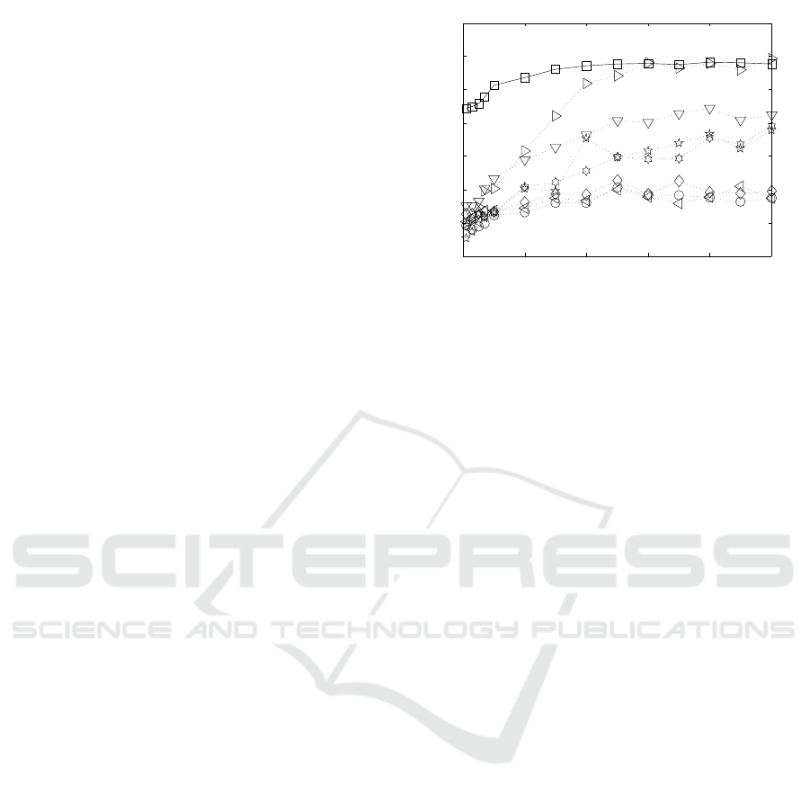
Figure 2 shows the resulting AUC score values as a
function of the percentage of attributes synthetically
perturbed by additive zero-mean Gaussian noise on
one out of the 10 datasets from Table 2. The x-
axis indicates the percentage of perturbed attributes
w.r.t. the total number of attributes, and the y-axis
shows the averaged AUC values over the 20 repeti-
tions of the experiment. As seen in the figure, the
proposed AAG method significantly outperforms the
other methods when the percentage of perturbed at-
tributes is lower than ≈ 40%. When the percentage
of perturbed attributes is higher than 40%, AAG per-
formance remains stable, and becomes comparable to
that of HiCS. Furthermore, it seems that AAG’s per-
formance is less affected by the percentage of per-
turbed attributes (i.e., lower variance in its AUC val-
ues), whereas the other methods are more affected.
Table 3 shows the averaged AUC values obtained
by the different subspace analysis methods, for all 10
datasets, when zero-mean Gaussian noise is added to
10% of the attributes. In each row of the table (i.e.
dataset), the AUC results obtained by the two best
subspace analysis methods are emphasized in Bold.
As seen from the Table, in all 10 datasets, AAG is
included in the list of two best performing subspace
analysis methods. In three cases, ENCLUS is in-
cluded with AAG in the two best performing meth-
ods, but in all of these thee cases, AAG outperforms
it. In four other cases, HiCS is included with AAG
in the list of two best performing methods, but only
in one of these cases it manages to outperform AAG.
CMI is also included two times with AAG in the list
of two best performing methods, but in all of these
seven cases, AAG outperforms it. All other methods
are left way behind.
0 0.2 0.4 0.6 0.8 1
0.1
0.2
0.3
0.4
0.5
0.6
0.7
0.8
Sensitivity resu lts for Features - Fourier AUC @ α ∈ [0, 1]
Factor of Number of Attributes
AUC
Figure 2: AUC as a function of the percentage of attributes
synthetically perturbed by additive zero-mean Gaussian
noise, for different subspace analysis methods. The sub-
space analysis methods are marked as follows: : AAG, C:
FB, B: HiCS, 5: ENCLUS, ◦: EWKM, ♦: AFG-k-means,
?: CMI, ∗: 4S.
Detecting Novelties
Table 4 shows the averaged AUC values obtained
under the novelty detection setting. Recall that the
reported values are the average over 20 repetitions.
Here as well, the two best results for each row (i.e.
dataset) are emphasized in Bold.
As seen from the table, in 8 out of the 10 datasets,
AAG is included in the list of two best performing
subspace analysis methods, and in 6 cases, it even
achieves the best performance. FB, seems to be the
second best method in the novelty detection setting,
reaching the list of the two best performing meth-
ods in 5 of the datasets, outperforming other state-
of-the-art subspace analysis methods such as HiCS
or 4S. HiCS and ENCLUS come next, both included
in the list of the two best performing methods two
times. 4S and CMI were found to be less effective
in detecting novelties, and were included in the list
of the two best performing methods twice and once
respectively. The soft subspace clustering (SSC) ap-
proaches EWKM and AFG-k-means were also found
to be less effective in detecting novelties. Interest-
ingly however, the SSC methods managed to achieve
relatively high AUC values in datasets with single-
type attributes such as Fourier, and Waveform. This is
most likely due to their use of the k-means algorithm.
In comparison to the previous experiment (i.e.,
Detecting Anomalies), the detection performance of
AAG is slightly less astonishing, and we attribute that
to the fact that in most of the analyzed datasets the
novelties seem to be “better” distributed along the en-
tire data space and henceforth, the performance of the
benchmark approaches became notably better.
To support our findings in Table 3 and Table 4,

Table 3: AUC performance results for ensemble of anomaly detection using MV-Set as local anomaly detection algorithm
(α ∈ [0.0,1.0]). Normal data samples were synthetically perturbed by additive zero-mean Gaussian noise in one subspace
comprising 10% of the total number of attributes i.e., p. The two best results are shown in Bold.
Dataset AAG FB HiCS ENCLUS EWKM AFG-k-means 4S CMI
Features-Fourier 0.613 0.256 0.370 0.294 0.147 0.202 0.238 0.244
Faults 0.759 0.484 0.424 0.564 0.448 0.550 0.594 0.601
Satimage 0.383 0.186 0.314 0.365 0.323 0.303 0.234 0.214
Arrhythmia 0.761 0.004 0.643 0.510 0.593 0.592 0.239 0.244
Pen Digits 0.725 0.402 0.293 0.627 0.543 0.524 0.241 0.301
Features-Pixels 0.693 0.497 0.381 0.452 0.474 0.365 0.504 0.533
Letters 0.664 0.289 0.564 0.640 0.425 0.337 0.416 0.419
Waveform 0.602 0.468 0.548 0.490 0.433 0.431 0.442 0.455
Sonar 0.546 0.246 0.499 0.373 0.232 0.299 0.391 0.405
Thyroid 0.843 0.252 0.750 0.289 0.236 0.591 0.632 0.470
we followed the statistical significance tests proposed
in (Dem
ˇ
sar, 2006). By applying the non-parametric
Friedman test in each table, we obtained the F-
statistics F = 35.025 and F = 55.945, respectively.
Based on the critical value of 3.245 at a significance
level of 0.05, the null-hypothesis can be rejected for
both experiments. The obtained statistical values for
the post-hoc tests between AAG to each one of the
benchmarked approaches, showed a p-Value ¡ 0.05 for
all cases, concluding that AAG outperforms all of its
competitors in the selected cases.
Detailed Comparison
The rest of this subsection provides a more detailed
comparison of AAG to the other benchmark ap-
proaches.
With respect to the FB approach, the results ob-
tained as anomaly detection ensemble reveals a rel-
atively low performance whereas for novelty detec-
tion ensembles it achieved, on average, comparable
results. Novel classes, as oppose to random noise,
manifest certain correlation among different attributes
that FB manages to detect. However, in more com-
plex datasets where attributes are of mixed nature, and
the data dimensionality is relatively high in compari-
son to the number of samples, FB’s performance de-
grades. A possible reason for this behavior can be at-
tributed to the different and higher sizes of subspaces,
since more data samples are needed to avoid the curse
of dimensionality (Scott, 1992).
Unlike HiCS, AAG succeeds in finding a smaller
number of subspaces that can be directly applied. The
reason for this lies in the search strategy of HiCS
which is based on the A-Priori approach and then ran-
domly permuting attributes to reduce the algorithm
complexity. HiCS retrieves several hundreds of sub-
spaces that afterwards have to be filtered in some fash-
ion. This can be observed from the obtained results in
the anomaly detection evaluation, where in average,
the HiCS method misses to find moderate deviations
in the dataset.
With respect to ENCLUS, although it does not re-
quire to set the number of generated subspaces in ad-
vance, it does require three other parameters as input,
such that their tuning requires an extensive grid search
over the support of the parameters. Opposite of FB,
we see that it performs better in the case of anomaly
detection applications but its performance degrades
as subspace method for novelty detection ensembles.
Finally, we note that ENCLUS presented the highest
training run-time for one of the evaluated sets of pa-
rameters.
The subspace clustering approaches EWKM and
AFG-k-means obtained the worst performance values
in anomaly as well as in novelty detection ensem-
bles. The poorer performance with respect to other
approaches, is due to the fact that attributes are dis-
carded from the set of subspaces. Consequently, nei-
ther novel nor abnormal samples can be efficiently
identified. Additionally, we found that it was not triv-
ial to set the number of clusters, a critical parame-
ter for both approaches. In both subspace clustering
methods, the number of clusters has the major im-
pact in the subspace selected when optimizing the ex-
tended k-means cost objective.
For their part CMI and 4S resulted in lower perfor-
mance than the proposed AAG, both for novelty and
for anomaly detection. Only in one case did both ap-
proaches manage to outperform all other benchmark
approaches. Whereas the 4S method requires to set
the maximal number of attributes, in CMI the num-
ber of clusters in the k-means turns out to be critical
for finding highly qualitative subspaces. This is mani-
fested in the obtained results for both evaluations, i.e.
anomaly and novelty detection ensembles.

Table 4: AUC performance results for ensemble of novelty detection using MV-Set as local anomaly detection algorithm
(α ∈ [0.0,1.0]). The two best results are shown in Bold.
Dataset AAG FB HiCS ENCLUS EWKM AFG-k-means 4S CMI
Features-Fourier 0.948 0.896 0.877 0.764 0.736 0.804 0.851 0.855
Faults 0.695 0.299 0.575 0.568 0.349 0.392 0.528 0.511
Satimage 0.989 0.979 0.920 0.882 0.836 0.840 0.814 0.809
Arrhythmia 0.653 0.187 0.573 0.605 0.348 0.496 0.574 0.554
Pen Digits 0.908 0.990 0.874 0.895 0.772 0.658 0.842 0.833
Features-Pixels 0.991 0.996 0.839 0.534 0.956 0.919 0.768 0.755
Letters 0.374 0.307 0.485 0.486 0.572 0.539 0.486 0.445
Waveform 0.896 0.853 0.799 0.731 0.843 0.804 0.824 0.831
Sonar 0.634 0.427 0.588 0.508 0.531 0.503 0.492 0.501
Thyroid 0.589 0.449 0.490 0.299 0.207 0.194 0.638 0.643
5.3 Run-time Evaluation
We have also evaluated the time taken to train each of
the ensembles on the 10 datasets used in this paper.
Table 5 shows the runtime results for the four bench-
mark methods that obtained the best detection results
in the previous two subsections (i.e., FB, HiCS, and
ENCLUS). Best results are shown in Bold.
As seen in Table 5, in the majority of the 10 stud-
ied cases, the ensemble using AAG as the subspace
analysis approach, finished its execution faster than
that using ENCLUS or HiCS. One reason for this
superiority is that AAG finds, on average, a smaller
number of subspaces than the other two competitors.
This is most likely due to the A-priori method that the
other two methods employ to search for subspaces,
as opposed to the Agglomerative approach that AAG
employs.
Table 5: Runtime evaluation (in seconds) of the training
phase for the ensembles based on AAG, FB, ENCLUS and
HiCS on the 10 datasets. Best result shown in Bold.
Dataset AAG FB HiCS ENCLUS
Fourier 316.5 146.4 317.8 5817.5
Faults 77.5 52.9 387.7 2166.7
Satimage 201.8 135.7 1370.2 1944.8
Arrhythmia 331.2 1863.8 1370.4 1540.9
Pen Digits 34.5 101.5 871.6 404.1
Pixels 826.4 6144.7 323.2 7122.3
Letters 278.5 123.1 1869.5 1236.5
Waveform 55.2 78.8 360.9 2694.5
Sonar 243.3 175.7 218.8 48667.8
Thyroid 162.8 855.9 1655.2 1862.9
6 DISCUSSION AND FUTURE
WORK
In this paper, we presented the Agglomerative At-
tribute Grouping (AAG) subspace analysis algo-
rithm that aims to find high-quality subspaces for
anomaly detection ensembles. Similar to other re-
cent state-of-the-art approaches for subspace analy-
sis, AAG searches for subspaces with highly corre-
lated attributes. To assess how correlative a sub-
set of attributes is, AAG uses a metric derived from
information-theory measures of partitions. Due to the
time complexity of the proposed metric with respect
to the number of attributes, we suggested a way to ap-
proximate the metric in cases where the number of at-
tributes is large. Equipped with the newly suggested
metric, AAG applies a variation of the well-known
agglomerative algorithm to search for highly corre-
lated subspaces. Our variation of the agglomerative
algorithm also applies a pruning rule that reduces re-
dundancy in the final set of subspaces.
As a result of combining the agglomerative ap-
proach with the suggested metric, AAG avoids any
tuning of parameters. Moreover, as our extensive
evaluation shows, AAG manages to outperform other
classical and state-of-the-art subspace analysis algo-
rithms when used as part of an anomaly detection
ensemble, both in its better ability to distinguish be-
tween normal and abnormal observations, as well as
with its fastest training time. Finally, as demonstrated
in our evaluation, AAG also outperforms other sub-
space analysis techniques when used as part of nov-
elty detection ensembles.
The AAG algorithm presented in this paper ad-
dresses the case where no separation is made between
normal observations (i.e., there is only one normal
class). In future work we aim to extend AAG to be
applicable for datasets with multi-class normal obser-
vations. While the trivial way of doing so, is to ap-
ply AAG on each one of the normal classes separately
and unify the sets of subspaces, we would like to uti-
lize the information available in the different classes
to find higher quality subspaces.

REFERENCES
Aggarwal, C. C. (2015). Outlier analysis. In Data Mining,
pages 237–263. Springer.
Aggarwal, C. C. and Yu, P. S. (2001). Outlier detection for
high dimensional data. pages 37–46.
Agrawal, R., Gehrke, J., Gunopulos, D., and Raghavan, P.
(1998). Automatic subspace clustering of high dimen-
sional data for data mining applications, volume 27.
ACM.
Agrawal, R., Srikant, R., et al. (1994). Fast algorithms for
mining association rules. 1215:487–499.
Bache, K. and Lichman, M. (2013). Uci machine learning
repository. http://archive.ics.uci.edu/ml.
Bajovic, D., Sinopoli, B., and Xavier, J. (2011). Sensor
selection for event detection in wireless sensor net-
works. IEEE Transactions on Signal Processing, 59.
Chandola, V., Banerjee, A., and Kumar, V. (2007).
Anomaly detection: A survey. Technical report, De-
partment of Computer Science and Engineering, Uni-
versity of Minnesota.
Cheng, C.-H., Fu, A. W., and Zhang, Y. (1999). Entropy-
based subspace clustering for mining numerical data.
In KDD, pages 84–93.
Cormen, T. H. (2009). Introduction to algorithms. MIT
press.
Cover, T. M. and Thomas, J. A. (2006). Elements of Infor-
mation Theory. John Wiley and Sons, Inc.
Dem
ˇ
sar, J. (2006). Statistical comparisons of classifiers
over multiple data sets. Journal of Machine Learning
Research, 7:1–30.
Deng, Z., Choi, K.-S., Jiang, Y., Wang, J., and Wang, S.
(2016). A survey on soft subspace clustering. Infor-
mation Sciences, 348:84–106.
Gan, G. and Ng, M. K.-P. (2015). Subspace clustering
with automatic feature grouping. Pattern Recognition,
48(11):3703–3713.
Gan, G., Wu, J., and Yang, Z. (2006). A fuzzy subspace
algorithm for clustering high dimensional data. pages
271–278.
Garc
´
ıa, S., Luengo, J., S
´
aez, J. A., L
´
opez, V., and Herrera,
F. (2014). A survey of discretization techniques: Tax-
onomy and empirical analysis in supervised learning.
IEEE Transactions on Knowledge and Data Engineer-
ing, 25(4):734–750.
Ge, Z. Q. and Song, Z. H. (2013). Multivariate Statistical
Process Control: Process Monitoring Methods and
Applications. Springer London Dordrecht Heidelberg
New York.
Goldstein, M. and Uchida, S. (2016). A comparative eval-
uation of unsupervised anomaly detection algorithms
for multivariate data. PloS one, 11(4):e0152173.
Jakulin, A. (2005). Machine learning based on attribute
interactions. Univerza v Ljubljani.
Jing, L., Ng, M. K., , and Huang, J. Z. (2007). An entropy
weighting k-means algorithm for subspace clustering
of high-dimensional sparse data. IEEE Transactios on
Knowledge and Data Engineering, 18(8):1026–1041.
Jyothsna, V., Prasad, V. V. R., and Prasad, K. M. (2011). A
review of anomaly based intrusion detection systems.
International Journal of Computer Applications.
Kagan, E. and Ben-Gal, I. (2013). Probabilistic Search for
Tracking Targets: Theory and Modern Applications.
John Wiley and Sons, Inc.
Kagan, E. and Ben-Gal, I. (2014). A group testing algorithm
with online informational learning. IIE Transactions,
46(2):164–184.
Keller, F., M
¨
uller, E., and B
¨
ohm, K. (2012). Hics: High
contrast subspaces for density-based outlier ranking.
In Proceedings of the 2012 IEEE 28th International
Conference on Data Engineering.
Kriegel, H.-P., Kr
¨
oger, P., and Zimek, A. (2009a). Clus-
tering high-dimensional data: A survey on subspace
clustering, pattern-based clustering, and correlation
clustering. ACM Transactions on Knowledge Discov-
ery from Data (TKDD), 3(1):1.
Kriegel, H.-P., Schubert, E., Zimek, A., and Kr
¨
oger, P.
(2009b). Outlier detection in axis-parallel subspaces
of high dimensional data. pages 831–838.
Kuratowski, C. (1961). Introduction to set theory and topol-
ogy.
Lazarevic, A. and Kumar, V. (2005). Feature bagging for
outlier detection. In ACM, editor, KDD’05.
Maimon, O. and Rockach, L. (2005). Data Mining and
Knowledge Discovery Handbook: A Complete Guide
for Practitioners and Researchers, chapter Outlier de-
tection. Kluwer Academic Publishers.
Markou, M. and Singh, S. (2003). Novelty detection: A
review?part1: Statistical approaches. Signal Process-
ing, 83:2481–2497.
McGill, W. J. (1954). Multivariate information transmis-
sion. Psychometrika, 19(2):97–116.
Menahem, E., Rokach, L., and Elovici, Y. (2013). Combin-
ing one-class classifiers via meta learning.
M
¨
uller, E., Schiffer, M., and Seidl, T. (2010). Adaptive out-
lierness for subspace outlier ranking. In CIKM, pages
1629–1632.
M
¨
uller, E., Schiffer, M., and Seidl, T. (2011). Statistical
selection of relevant subspace projections for outlier
ranking. In 2011 IEEE 27th International Conference
on Data Engineering.
Nguyen, H. V., M
¨
uller, E., and B
¨
ohm, K. (2013a). 4s: Scal-
able subspace search scheme overcoming traditional
apriori processing. IEEE International Conference on
Big Data, pages 359–367.
Nguyen, H. V., M
¨
uller, E., Vreeke, J. ans Keller, F., and
B
¨
ohm, K. (2013b). Cmi: An information-theoretic
contrast measure for enhancing subspace cluster and
outlier detection. SIAM.
Park, C., Huang, J. Z., and Ding, Y. (2010). A computable
plug-in estimator of minimum volume sets for novelty
detection. Operation Research, Informs.
Parsons, L., Haque, E., and Liu, H. (2004). Subspace
clustering for high dimensional data: a review. Acm
Sigkdd Explorations Newsletter, 6(1):90–105.
Pimentel, M. A. F., Clifton, D. A., Clifton, L., and
Tarassenko, L. (2014). A review of novelty detection.
Signal Processing, 99:215–249.

Rokhlin, V. A. (1967). Lectures on the entropy theory of
measure-preserving transformations. A Series Of Ar-
ticles On Ergodic Theory.
Scott, D. W. (1992). Multivariate Density Estimation - The-
ory, Practice, and Visualization. John Wiley and Sons,
Inc.
Simovici, D. (2007). On generalized entropy and entropic
metrics. Journal of Multiple Valued Logic and Soft
Computing, 13(4/6):295.
Steinwart, I., Hush, D., and Scovel, C. (2006). A classifi-
cation framework for anomaly detection. Journal of
Machine Learning Research, (6):211–232.
Watanabe, S. (1960). Information theoretical analysis of
multivariate correlation. IBM Journal of research and
development, 4(1):66–82.
