Metaheuristic Solutions for Solving Controller Placement Problem in

SDN-based WAN Architecture

Kshira Sagar Sahoo

, Anamay Sarkar

, Sambit Kumar Mishra

, Bibhudatta Sahoo

, Deepak Puthal

2,†

Mohammad S. Obaidat

3,4,†,‡

and Balqies Sadun

National Institute of Technology, Rourkela, India

University of Technology Sydney, Australia

Fordham University, U.S.A.

University of Jordan, Jordan

Al-Balqa Applied University, Jordan

Keywords:

SDN, Controller, CPP, FireFly, PSO.

Abstract:

Software Deﬁned Networks (SDN) is a popular paradigm in the modern networking systems that decouples

the control logic from the underlying hardware devices. The control logic has implemented as a software com-

ponent and residing in a server called controller. To increase the performance, deploying multiple controllers

in a large- scale network is one of the key challenges of SDN. To solve this, authors have considered con-

troller placement problem (CPP) as a multi-objective combinatorial optimization problem and used different

heuristics. Such heuristics can be executed within a speciﬁc time-frame for small and medium sized topology,

but out of scope for large scale instances like Wide Area Network (WAN). In order to obtain better results,

we propose Particle Swarm Optimization (PSO) and Fireﬂy two population-based meta-heuristic algorithms

for optimal placement of the controllers, which take a particular set of objective functions and return the best

possible position out of them. The problem has been deﬁned, taking into consideration both controllers to

switch and inter-controller latency as the objective functions. The performance of the algorithms evaluated

on a set of publicly available network topologies in terms execution time. The results show that the FireFly

algorithm performs better than PSO and random approach under various conditions.

1 INTRODUCTION

In recent years, the use of Software Deﬁned Net-

working (SDN) has become an emerging technology

that provides many advantages to the cloud data cen-

ters and network service providers. Both SDN and

Network Function Virtualization (NFV) technology

creates the new era of network innovation through

the virtualization of network resources (Jarraya et al.,

2014),(Jammal et al., 2014). The underlying principle

of SDN is the abstraction of the control plane from

the data plane. It introduces the logically centralized

control plane also referred to as Network Operating

System (NOS), that hides the network complexities to

the application developer by introducing well known

southbound APIs. The network intelligence moved

†

Fellow of IEEE & Fellow of SCS

‡

Corresponding author

onto one or more external servers from the hardware

devices, called controllers, which has a global view of

the entire network(Sahoo et al., 2016).

Although placing a single controller is economi-

cally advantageous, it suffers single point of failure.

Hence, deploying multiple controllers in the network

is an alternate solution. However, random placing of

controllers affects the performance of the system and

degrades end to end QoS. So, it requires a proper plan-

ning to ﬁnd the optimal location of the controller to

get satisfactory performance and a reliable SDN. The

CPP is an optimization problem is similar to facility

location problem; which has considered as a NP-hard

problem. Authors in (Heller et al., 2012), shows the

performance of the network by varying the position of

the controller in the network. So, it is a big challenge

to ﬁnd the location as well as number of controllers to

be deployed in the network. Dynamically changing

Sahoo, K., Sarkar, A., Mishra, S., Sahoo, B., Puthal, D., Obaidat, M. and Sadun, B.

Metaheuristic Solutions for Solving Controller Placement Problem in SDN-based WAN Architecture.

DOI: 10.5220/0006483200150023

In Proceedings of the 14th International Joint Conference on e-Business and Telecommunications (ICETE 2017) - Volume 1: DCNET, pages 15-23

ISBN: 978-989-758-256-1

the network architecture especially for WAN is a chal-

lenging task for the network operator. To adapt to this

dynamics; the optimized location needs to be calcu-

lated. The POCO (Hock et al., 2014) framework has

capable of handling small and medium size topology

which provide the solution within seconds.However,

for the large-scale network, it requires a lot of time for

exhaustive evaluation for ﬁnding the location which

may not cope with the dynamics of the network. The

summary of our contributions are as follows:

• The main objective of this work is to minimize

controller to node and inter-controller latency in

the average and worst case scenario.

• To best of our knowledge, we are the ﬁrst to

propose the population-based meta-heuristic tech-

niques to solve CPP on a set of real topologies

considering the above as the objective function.

The rest of this paper has organized as follows. The

Section II introduced the related work; the mathemat-

ical formulation described in Section III. The con-

sidered meta-heuristics algorithms have discussed in

Section IV. Then Section V exhibits the performance

analysis during the experiment followed by conclu-

sion in Section VI.

2 RELATED WORK

In a given network which comprises of certain

nodes(node may be switch, router, ﬁrewall etc.) , how

to place the controllers is an open question. At ﬁrst,

Heller et al.(Heller et al., 2012) examined both aver-

age and worst case latency between the switch and

controller in the Internet2 topology. The latency and

trafﬁc load between switch and controller have em-

phasized by Yao (Yao et al., 2014). In another work,

Bari (Bari et al., 2013), proposed a dynamical provi-

sioning of controllers aims to reduce ﬂow set-up time

and reassignment time of a switch to another con-

troller in case of an overloaded situation. The POCO

framework has been formulated with different met-

rics. The trade-off between the different metrics with

all possible placements is examined in POCO. Al-

though the inter-controller latency has considered it

has not discussed in-depth in their work. In his work

Lange et la.(Lange et al., 2015) extends the POCO

framework and deploy K controller in the dynamic

topologies. In their work, they have used Pareto Sim-

ulated Annealing (PSA) a meta-heuristic to solve the

CPP. Hu et la. (Hu et al., 2013) worked on the re-

liability of the controller. They have used a met-

ric to quantify the reliability called expected percent-

age of control path loss but ignores inter-controller

latency. The paper(Sallahi and St-Hilaire, 2015),

solve the CPP with various multi-objective functions.

To the best of our knowledge, the authors have not

used any population-based meta-heuristic technique

in their work.

3 PROBLEM FORMULATION

In this work, we represent the network as a graph

G(V,E), where V and E represent as the node set

and edge set. The node set consists of the switch,

router, and controllers. In SDN, the switches and con-

trollers are the forwarding elements. Here, we as-

sumed that the controller locations are some of the

forwarding nodes. Let d(v,c) is the shortest path dis-

tance from a forwarding node v ∈ V to one of the con-

troller c ∈ C. For a particular placement the number

of controllers is ﬁxed to k, i.e. |C

| = k. The all pos-

sible controller placement set can be represented as

C = {C

,...,C

}. For ﬁnding out a location for

the controller c

∈ C

; can be set as an optimization

problem where the evaluation metrics are optimized.

In our work, we have used latency as the evaluation

metric. Latency refers to the time taken to reach a

packet from source node to the destination node. But

in case of SDN, the propagation latency between node

and controller is proportional to the distance between

a node to controller.

3.1 Controller to Switch Latency

It is the most common metric used in CPP. It is the

longest distance between a node (v

) and a controller

) i.e. max d(v

). This is considered as the worst-

case switch to controller latency. The objective of this

worst case latency is to minimize the longest distance.

worstlat

v∈V

max

c∈C

d(v,c) (1)

For the average latency case, the average distance be-

tween the placed controllers and remaining nodes as-

signed to them is calculated. In order tocompute it,

the following equation has used.

avglat

|V |

∑

v∈V

min

c∈C

d(v,c) (2)

3.2 Inter-controller Latency

The latency between the individual controllers has a

major signiﬁcance because communications between

these controllers are required to achieve proper syn-

chronization of the network state. In order to mini-

mize the controller to controller communication cost,

DCNET 2017 - 8th International Conference on Data Communication Networking

they should deploy near to each other. To compute

this metric, the d

must be calculated. The new

) is produced from d(i, j) that signiﬁes the

shortest distance between controller c

to controller

. The matrix d

removes the node that does not hold

as a controller. The following equation is used to cal-

culate the above metric.

avgiclat

|k|

∑

∈C

min d(c

) (3)

For worst-case inter-controller latency the maxi-

mum distance that separates controllers is computed.

The considered metric can be formulated as:

worsticlat

∈C

d(c

) (4)

4 META-HEURISTIC

TECHNIQUES FOR CPP

PROBLEM

With a given the number of controllers k to be de-

ployed in the network, the goal of our work is to ﬁnd

a placement C

from the set C, such that the consid-

ered metrics must be minimized.

The single state meta-heuristic techniques like

simulated annealing (SA) has a single candidate so-

lution. This solution is used to compare with possible

new solutions. Population-based algorithms like Fire-

ﬂy, PSO store many candidate solutions and the solu-

tion set compare them against each other. For explor-

ing large and continuous space regions, single state

algorithms are not suitable for large search space be-

cause of the possibility of stuck in local optima and

lack of comparisons between candidate solutions.

4.1 PSO Algorithm for CPP

Particle Swarm Optimization (PSO) is a population-

based stochastic technique. This algorithm searches

the optimum solution from a population called the

swarm. Based on two types of learning i.e. cogni-

tive and social learning; it ﬁnds the best solution out

of many. At the initial phase cognitive factor required

for determining the best position. After searching the

local best, social factor helps to ﬁnd the global best

position.

Let there are n particles, that represent the poten-

tial solutions and each particle represented as a d-

dimension vector. Let, the current position of the

particle is χ

= [x

,...,x

], where i ∈ 1...n. The

current velocity is V

= v

,...,v

. The best posi-

tion of the particle P

is p

, p

,..., p

. The P

is the

global best position vector.

At the time t +1, it updates the position (χ

t+1

) and

velocity (V

t+1

) of the individual particle is deﬁned as

follows:

t+1

= ωV

+ c1

r1(P

− χ

) + c2

r2(P

gbd

− χ

)

(5)

t+1

= χ

+t (6)

Where ω represents initial weight,r1 and r2 denotes

the random sequence: r1,r2 ∈ {0, 1}. The positive

constant c1

and c2

adjusts the cognitive part and so-

cial part respectively. The value of ω is used for im-

proving the performance of the algorithm. The adap-

tive adjustment of ω helps to improve the local as well

as global search ability, which can be represented as:

ω = ω

max

−

max

− ω

min

max

× I (7)

In the Equation 7, I

max

represents the maximum num-

ber of iteration it can hold and I represents the current

iteration. The ω

max

and ω

min

represents the maximum

weight and minimum weight respectively.

4.2 Algorithm for CPP PSO

The CPP PSO Algorithm takes the co-ordinates

of the nodes (latlng), required number of

controllers(nCont), and the matrix containing

the shortest path from each node to all other nodes

(srtPathMtrx)as the inputs.The algorithm produces

the semi-optimized value (bstCst) of the cost function

and the ﬁnal location of the Controllers ( f nlPosPSO).

The algorithm begins by setting the number of

Nodes (numNod), x and y-co-ordinates of latlng

as latlngX and latlngY , initializing the number

of maximum iterations (maxIt), the population of

the swarm (nPop), inertia coefﬁcient (ω), damping

ratio for inertia coefﬁcient (ωdamp), individual

(c1) and social (c2) acceleration coefﬁcients and

sets Global Best Cost (glBest.Cst) to inﬁnity. It

initializes each particle’s position (par(i).Pos) as

a random permutation of nCont out of numNode.

Each particle’s velocity in x (par(i).Vel.x) and y

(par(i).Vel.y) components set to zeros. Also it

initializes each particle’s cost (par(i).Cst) using the

objective function. It also initializes best position of

each particle (par(i).Bst.Pos) as the current position

and best cost(par(i).Bst.Cst) as the current cost and

sets Global Best Cost(glBest.Cst) as the optimum

value among all the particles and Global Best Position

( f nl pos PSO) as the position of the particle giving

the optimal value. For each iteration and for the each

particle the Algorithm 2 updates the particle’s x and

y component of velocity and the position. With the

current position of the particle, x and y component of

velocity and latlng are given as input and updates the

Metaheuristic Solutions for Solving Controller Placement Problem in SDN-based WAN Architecture

Algorithm 1 CPP PSO

Input: latlng, nCont,srtPathMtrx

Output: optimized cost (bstCst), Final position of controllers ( f nlPosPSO)

Initialization :

1: numNod ← Size of latlng

2: latlngX , latlngY ← x- and y- co-ordinates of latlng

3: maxIt ← maximum number of iterations

4: nPop ← Swarm Size

5: w ← inertia coefﬁcient

6: wdamp ← damping ratio

7: c1 ← personal acceleration coefﬁcient

8: c2 ←social acceleration coefﬁcient

9: glBest.Cst ←Set Global Best Cost to ∞

10: for i = 1 to nPop do

11: par(i).Pos ←Randomly select nCont positions from numNodes

12: par(i).Vel.x ←Initialize x-component of velocity with 0

13: par(i).Vel.y ←Initialize y-component of velocity with 0

14: par(i).Cst ← Pass par(i).Pos,latlngX , srtPathMtrx to CST NC

15: par(i).Bst.Pos ← par(i).Pos

16: par(i).Bst.Cst ← par(i).Cst

17: if (par(i).Bst.Cst < glBest.Cst) then

18: glBest.Cst ← par(i).Bst.Cst

19: f nl pos PSO ← par(i).Pos

20: end if

21: end for

22: BstCost ←Initialize the Best Cost with 0

Optimization Loop

23: for it = 1 to maxIt do

24: for i = 1 to nPop do

25: par(i).Vel.x ←Update x component using Equation 5

26: par(i).Vel.y ← Update y component of velocity similar to x

component of velocity

27: par(i).Pos ← Pass

par(i).Pos, par(i).Vel.x, par(i).Vel.y,latlngX , latlngY to

updPos PSO

28: par(i).Cst ← Pass par(i).Pos,latlngX , srtPathMtrx to CST NC

29: if (par(i).Cst < par(i).Bst.Cst) then

30: par(i).Bst.Pos ← par(i).Pos

31: par(i).Bst.Cst ← par(i).Cst

32: if (par(i).Bst.Cst < glBest.Cst) then

33: glBest.Cst ← par(i).Bst.Cst

34: f nlPosPSO ← par(i).Pos

35: end if

36: end if

37: end for

38: BstCost(it) ← glBest.Cst

39: w ← w × wdamp

40: end for

41: z ← BstCost from last iteration

42: return z, f nlPosPSO

cost of the particle using the considered objective

function. If the new cost is better than the previous

cost of the particle, update the particle’s current po-

sition and cost. If the updated cost is better than the

previous one then, the global best cost and global best

positions are updated to the particle’s cost and posi-

tion respectively.

The updPos CPP PSO Algorithm takes the cur-

rent position of the particle (x), x-component of veloc-

ity (vx), y-component of velocity (vy) , x-coordinates

of all nodes (latlngX) and y-coordinates of all nodes

(latlngY ) as input and produces the updated posi-

tion (z). In order to obtains the x-component of

particle’s i

controller position (xPos(i)), this al-

gorithm get the sum of x-coordinate of i

con-

troller (latlngX(x(i))) and x-component of velocity

of i

particle (vx(i)). This process is similar for

the y-component of particle’s i

controller position

(yPos(i)). For each controller location, it initializes

minimum distance between ﬁnal position and any ac-

tual node co-ordinate (mini) to inﬁnity and initializes

the index (mini index) of such a node to 0. Then,

for each controller location, it checks all other nodes

and updates mini index as the index of the node which

gives minimum distance.

Algorithm 2 updPos CPP PSO

Input: x,vx, vy,latlngX,latlngY

Output: updated position (z)

Initialization :

1: sze ←size of x

2: numNode ← size of latlngX

3: xPos ←Initialize the x component of position with zero

4: yPos ←Initialize the y component of position with zero

5: dist←Initialize the ﬁnal location with 0s

Main Body

6: for i = 1 to sze do

7: xPos(i) ← latlngX (x(i)) + vx(i)

8: yPos(i) ← latlngY(x(i)) + vy(i)

9: end for

10: for i = 1 to sze do

11: mini ← ∞

12: mini index ← 0

13: for j = 1 to numNode do

14: if (Distance between i

position and j

node is less than mini)

then

15: mini← Distance between i

position and j

node

16: mini index ← j

17: end if

18: end for

19: dist for i

iteration ← mini index

20: end for

21: z← dist

22: return z

4.3 Fireﬂy Algorithm (FFA)

This Algorithm 3 is based on the ﬂashing characteris-

tics of the ﬁreﬂies. The biochemical process of illu-

minating light from ﬁreﬂy is called bio-luminescence

has a signiﬁcance role. The basic objective of this al-

gorithm is to attract the opponent through rhythmic

ﬂashes. The inverse squared law inferred that the in-

tensity of the light(I) decreases as the distance r in-

creases. So, in a simple form the FFA based on the

equation 8.

I ∝

(8)

DCNET 2017 - 8th International Conference on Data Communication Networking

The light intensity (I)is having a ﬁxed absorption co-

efﬁcient γ, which has given in the equation 9.

I = I

−rγ

(9)

Where, I

is the initial light intensity. For simplicity

and to avoid singularity at r = 0, we can combine both

the equations.

I = I

−r

(10)

The attractiveness (β) is directly proportional to the

intensity of the light, that are coming from nearby

ﬁreﬂies, which has given in the below equation.

β = β

−r

(11)

In the Equation 11 β

is the attractiveness at r = 0.

For faster calculation we normalize the equation as a

monotonically decreasing function.

β = β

−r

;(m ≥ 1) (12)

The movement of one butterﬂy(i) to another butterﬂy

( j) is determined by the given equation 13

= x

+ β

i j

− x

) + αε

(13)

The third term is used for randomization where, α is

the randomized parameter and ε

is the vector of ran-

dom numbers.

4.4 Algorithm for CPP FFA

The Algorithm 3 takes the co-ordinates of the nodes,

number of controllers and the matrix containing the

shortest path from each node to all other nodes as in-

put. Similar to CPP PSO it produces the optimized

value of the cost function and the ﬁnal location of the

controllers.

The Algorithm 4 takes all the ﬁreﬂies (par), light

intensity of the ﬁreﬂy (Lightn), randomness coefﬁ-

cient (α), absorption coefﬁcient (γ) , x co-ordinates

of nodes (latlngX) and y co-ordinates of the nodes

(latlngY) as inputs. It returns the updated position of

all the ﬁreﬂies (par). The algorithm begins by ini-

tializing the number of nodes (numNode), number

of particles (numPar) and the number of controllers

(numCon) as the size of any particle. For each con-

troller (numCon) the following steps are performed.

It sets the x-coordinate (xo) and y-coordinate (yo) of

all ﬁreﬂies for all controllers to zeros. Then the x-

coordinate (xo(i)) and y-coordinate of each particle

(yo(i)) are updated. For each particle, set r as the dis-

tance between i

particle and j

particle. If the light

intensity of i

particle (Lightn(i)) is greater than the

light intensity of j

particle (Lighto( j)), then set β as

the negative exponent of product of γ and r. The pa-

rameter xn(i) set as in per the equation 13. Finally the

algorithm sets dist as the updated position of the ﬁre-

ﬂies, in terms of the indices of the corresponding

Algorithm 3: CPP FFA.

Input: latlng, nCont,avlPathMtrx, srtPathMtrx

Output: bstCst, f nlPosFire

Initialization :

1: numNode ← size o f latlng

2: latlngX ← x co − ordinates o f latlng

3: latlngY ← y co − ordinates o f latlng

4: nPop ←Initialize number of ﬁreﬂies

5: maxGen ←Initialize number of iterations

6: α ←Set the randomness coefﬁcient

7: γ ←Set the absorption coefﬁcient

8: δ ←Set the randomness reduction coefﬁcient

9: minCst ←Initialize the minimum cost of objective function to inﬁnity

10: Lightn ←Initialize the light intensity of all the ﬁreﬂies to zeros

11: for i = 1 to nPop do

12: par(i).Pos ←Randomly select nCont from numNode

13: end for

Optimization Loop

14: for i = 1 to maxGen do

15: zn ←Initialize the cost for all the ﬁreﬂies with zeros

16: for j = 1 to nPop do

17: zn( j) ←Pass par( j).Pos,latlngX,srtPathMtrx to Objective

function

18: end for

19: [Lightn] ← Return sorted zn in Lightn

20: Lighto ← Make a copy of Lightn

21: par ← Pass par,Lightn, Lighto,α, γ,latlngX,latlngY to

updPos Fire()

22: α ← α∗ δ

23: if (minCst > Lighto(1)) then

24: mincost ← Lighto(1)

25: f nlPosFire ←Set f nlPosFire as the position of ﬁreﬂy that gave

the minimum Cost

26: end if

27: end for

28: bstCst ← minCst;

29: return bstCst, f nlPosFire

controller location and then it sets each ﬁreﬂy’s cor-

responding controller location (par(g).Pos(k)).

4.5 Algorithm for the Cost Functions

In the main body of the algorithm, the average con-

troller latency is added with average inter-controller

latency. Average node latency and average controller

latency are added to obtain the objective function (z),

which is returned by the Algorithm 6.

5 EXPERIMENT

To evaluate of this work, we have taken various

topologies from the TopologyZoo website. As per

our knowledge since, no one has used any population-

based meta-heuristic technique to solve CPP problem.

In this work, we have used two metrics, which have

been already discussed in the previous section.

Metaheuristic Solutions for Solving Controller Placement Problem in SDN-based WAN Architecture

Algorithm 4: updPos FireFly.

Input: par, Lightn,Lighto, α,γ, latlngX,latlngY

Output: par

Initialization :

1: numNode ← size o f latlng

2: numPar ← size o f par

3: numCon ←Set number of controllers as size of any particle

Main Body

4: for k = 1 to numCon do

5: xo ←Initialize x-coordinates of the ﬁreﬂies by zeros

6: yo ←Initialize y-coordinates of the ﬁreﬂies by zeros

7: for i = 1 to numPar do

8: xo(i) ←Set the x-coordinate of ith particle’s kth controller loca-

tion from latlngX

9: yo(i) ←Set the y-coordinate of ith particle’s kth controller loca-

tion from latlngY

10: end for

11: xn ← xo

12: yn ← yo

13: for i = 1 to numPar do

14: for j = 1 to numPar do

15: r ←Distance between ith and jth particle

16: if (Lightn(i) > Lighto( j)) then

17: β ←Set as the negative exponent of product of γ and r

18: xn(i) ←Set as the sum of (product of previous xn(i) and

1 − β) and (product of previous xo( j) and β) and (product

of α and a random number)

19: yn(i) ←Set as the sum of (product of previous yn(i) and

1 − β) and (product of previous yo(j) and beta) and (prod-

uct of α and a random number)

20: end if

21: end for

22: end for

23: dist ←Initialize the ﬁnal location of k

controller of all ﬁreﬂies with

24: for i = 1 to numPar do

25: mini ← Initialize with in f inity

26: mini index ← Initialize with 0s

27: for j = 1 to numNode do

28: if (Distance between i

particle’s k

controller location and

node is less than mini) then

29: mini ← Distance between i

particle’s k

controller lo-

cation and j

node

30: mini index ← j

31: end if

32: end for

33: dist f or i

iteration ← mini index

34: end for

35: for g = 1 to numPar do

36: par(g).Pos(k) ← Set the g

particle’s k

controller location as

entry of dist

37: end for

38: end for

39: return par

All the algorithms are written in Matlab version

R2014a and runs on a system having Intel Core i5

with 4-Core processors and 8 GB RAM with Ubuntu

13.10 of 64-bit Operating System. The results are

obtained by running the algorithms 30 times on the

graph. Among 261 networks in the Topology-Zoo,

Algorithm 5: CST NC.

Input: x,latlngX,srtPathMtrx

Output: z

Initialization :

1: sze ←Set number of Controllers as the size of x

2: numNode ←Set number of Nodes as the size of latlngX

3: contLat ←Initialize average controller latency with 0

4: nodeLat ← Initialize average node latency with 0

Main Body

5: for i = 1 to sze do

6: for j = 1 to sze do

7: contLat ← contLat + srtPathMtrx(x(i), x( j))

8: end for

9: end for

10: contLat ← contLat/(sze ∗ sze)

11: for i = 1 to numNode do

12: mini ← ∞

13: for j = 1 to sze do

14: mini ← min(mini,srtPathMtrx(i,x( j)))

15: end for

16: nodeLat ← nodeLat + mini

17: end for

18: z ← nodeLat + contLat

19: return z

Algorithm 6: CST NC.

Input: x,latlngX,srtPathMtrx

Output: z

Initialization :

1: sze ←Set number of Controllers as the size of x

2: numNode ←Set number of Nodes as the size of latlngX

3: contLat ←Initialize average controller latency with 0

4: nodeLat ← Initialize average node latency with 0

Main Body

5: for i = 1 to sze do

6: for j = 1 to sze do

7: contLat ← contLat + srtPathMtrx(x(i), x( j))

8: end for

9: end for

10: contLat ← contLat/(sze ∗ sze)

11: for i = 1 to numNode do

12: mini ← ∞

13: for j = 1 to sze do

14: mini ← min(mini,srtPathMtrx(i,x( j)))

15: end for

16: nodeLat ← nodeLat + mini

17: end for

18: z ← nodeLat + contLat

19: return z

we have considered 20 topologies for our work. The

network sizes range from 50 to 150 nodes and among

them the total number of controllers considered are

between 5 to 20. The TataNld topology has been cho-

sen as an example, which contains 144 nodes and 141

edges. When more than one metric are optimized, it

is usually difﬁcult to ﬁnd an exact solution that satis-

ﬁes all at the same time. So, there is a trade-off that is

required between these two or more metrics. Thus to

justify the necessity, the Pareto frontier is used.

DCNET 2017 - 8th International Conference on Data Communication Networking

5.1 How Worthwhile to Optimize the

Controller Position?

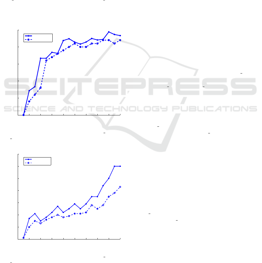
The Fig.1 and 2 shows the ratio of random deploy-

ment of the controller to our proposed algorithms on

the same topology. It has clearly observed that the av-

erage latency of the proposed algorithms is about 1.7

times greater than random deployment. For the larger

value of K(18), the cost of the random placement is

almost 70% higher than that of other placements. For

the worst case latency, this cost is even larger for

both the algorithms. The ratio starts from 1.5 for a

single controller, but for the higher value of K, the

CPP FFA increases to 2.1x, whereas CPP PSO in-

creases to 1.9x. Hence, it is important to optimize the

placement of controllers in a given topology.

0 2 4 6 8 10 12 14 16 18

1.5

1.55

1.6

1.65

1.7

1.75

Number of Controllers

ratio

CPP_FIREFLY

CPP_PSO

Figure 1: Ratio of random deployment to CPP PSO and

CPP FFA (Average-case).

0 2 4 6 8 10 12 14 16 18

1.5

1.6

1.7

1.8

1.9

2.1

2.2

Number of Controllers

ratio

CPP_FIREFLY

CPP_PSO

Figure 2: Ratio of random deployment to CPP PSO and

CPP FFA (Worst-case).

5.2 Performance of the Algorithms

The Fig. 3 and Fig. 5 analyzes the impact of average

and maximum latency on increasing the number of the

controller, k ranges from 1 to 20, under the same net-

work topology. The experimental result shows that by

increasing the number of controllers for each place-

ment, the both the latencies (cost) is decreased as ex-

pected. The average latency is calculated using both

Equation 2 and Equation 3. From the plot it can be

observed that, when k > 15 both average and worst

case latency are almost linear,so we restrict the num-

ber of controllers to 15 for the topology. Similar to

average case the worst case inter-controller latency is

computed using Equations 1 and 4. The average de-

lay of both meta-heuristic algorithms is usually rela-

tively more stable than random algorithm. When K

=16, the cost within an acceptable range for both the

algorithms,

5.3 Computational Time of the

Proposed Algorithms

With the increasing number of controller it can be

seen from the Fig. 4 and Fig. 6 that CPP FFA al-

gorithm takes the shortest time. The processing time

of both CPP FFA and CPP PSO is much faster than

random algorithm. Due to the randomness and non-

uniformity nature, the random algorithm behaves like

it. But, the execution time taken by the two meta-

heuristic techniques is almost close to each other in

both the cases. For the larger network like TataNld,

the CPP FFA algorithm converges to the optimal so-

lution slightly faster than CPP PSO.

5.4 Optimal Positions of the Controllers

Now, we compare the geographic locations of the

controllers with respect to the different objective

functions. The Fig. 7 and Fig. 8 shows the ﬁnal out-

come of the simulation with 15 controllers on TataNld

topology. The black circle represents the controller

position and the white circle represents the other than

controller. The Fig. 7 depicts the locations of the

controller that minimizes the average latency using

CPP FireFly algorithm, and the Fig. 8 represents the

same using CPP PSO algorithm.

6 CONCLUSIONS

In this paper, we discuss the controller placement

problem for SDN-based WAN architecture. The

greedy and brute force methods are well suited for

Metaheuristic Solutions for Solving Controller Placement Problem in SDN-based WAN Architecture

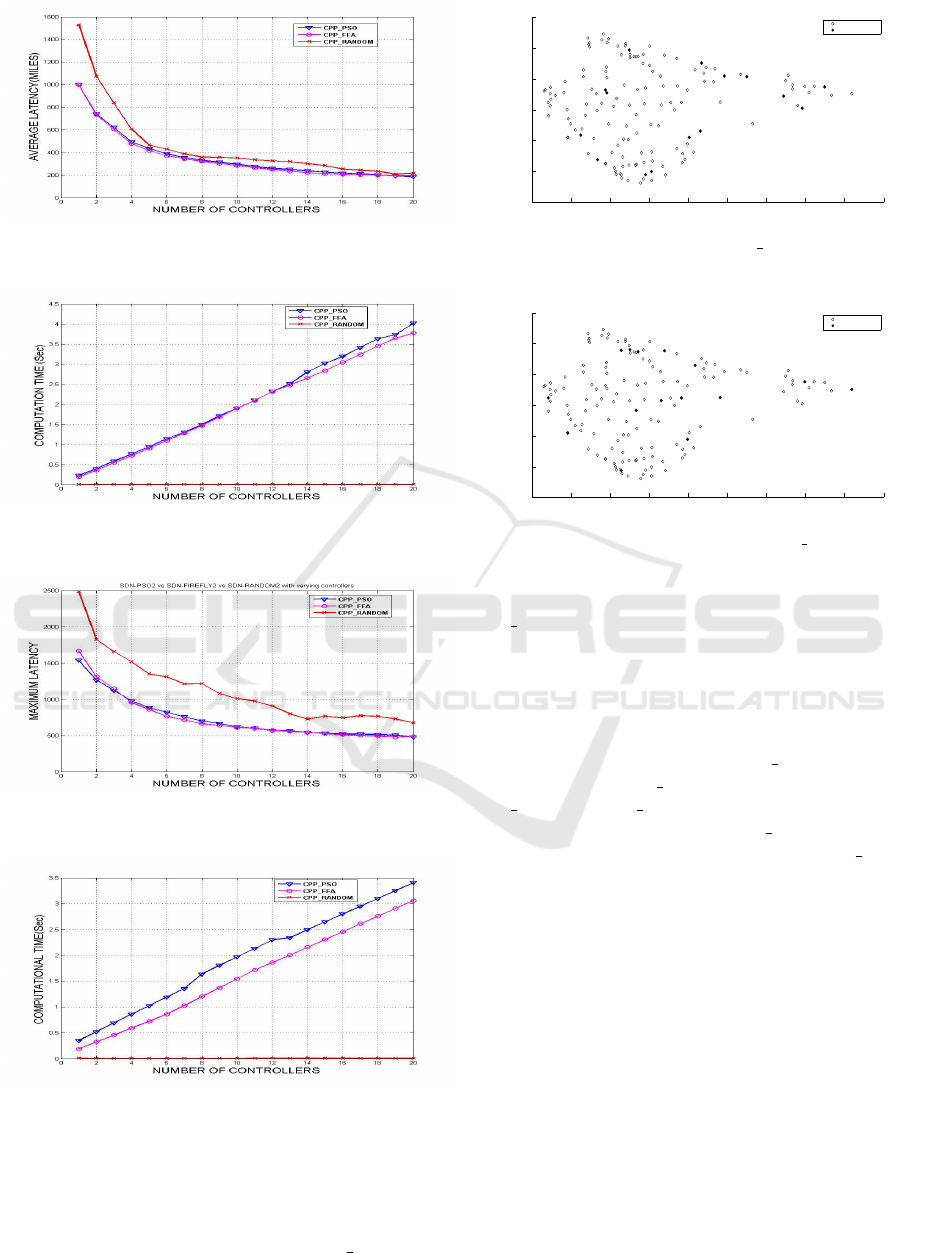
Figure 3: Impact of average case latency on deploying con-

trollers.

Figure 4: In average case the computational time of the al-

gorithms.

Figure 5: Impact of worst-case latency on deploying con-

trollers.

Figure 6: In worst case the computational time of the algo-

rithms.

small and medium-sized problem instances, but for

large scale problem instances a heuristic mecha-

nism is a wise choice. Hence, we propose two

meta-heuristic algorithms named as CPP PSO and

72 74 76 78 80 82 84 86 88 90

Longitude

Latitude

Other nodes

Controller Locations

Figure 7: Optimal placement using CPP FFA in the TataNld

(Average-case latency).

72 74 76 78 80 82 84 86 88 90

Longitude

Latitude

Other nodes

Controller Locations

Figure 8: Optimal placement using CPP PSO in the

TataNld (Average-case latency).

CPP FFA for evaluating CPP. In particular, such al-

gorithms optimize a set of objectives that ﬁnd the

optimal number and location of the controller. The

objective of this work is to minimize the latency

between controllers as well as from switch to con-

trollers. Experimental results show that for average

case and worst case latency, the CPP FFA has better

performance than CPP PSO. The time taken by both

CPP PSO and CPP FFA are in almost close level.

When network size is larger, CPP FFA converges

to the optimal solution slightly faster than CPP PSO

as it is the inherent property of these Meta-heuristic

techniques. Finally, the scope of this paper is not lim-

ited to only this two objectives. As future work, we

plan to incorporate other objective functions like load

balancing and multi-path connectivity.

REFERENCES

Bari, M. F., Roy, A. R., Chowdhury, S. R., Zhang, Q.,

Zhani, M. F., Ahmed, R., and Boutaba, R. (2013). Dy-

namic controller provisioning in software deﬁned net-

works. In Network and Service Management (CNSM),

2013 9th International Conference on, pages 18–25.

IEEE.

Heller, B., Sherwood, R., and McKeown, N. (2012). The

controller placement problem. In Proceedings of the

DCNET 2017 - 8th International Conference on Data Communication Networking

ﬁrst workshop on Hot topics in software deﬁned net-

works, pages 7–12. ACM.

Hock, D., Gebert, S., Hartmann, M., Zinner, T., and Tran-

Gia, P. (2014). Poco-framework for pareto-optimal

resilient controller placement in sdn-based core net-

works. In Network Operations and Management Sym-

posium (NOMS), 2014 IEEE, pages 1–2. IEEE.

Hu, Y., Wendong, W., Gong, X., Que, X., and Shiduan,

C. (2013). Reliability-aware controller placement for

software-deﬁned networks. In Integrated Network

Management (IM 2013), 2013 IFIP/IEEE Interna-

tional Symposium on, pages 672–675. IEEE.

Jammal, M., Singh, T., Shami, A., Asal, R., and Li, Y.

(2014). Software deﬁned networking: State of the art

and research challenges. Computer Networks, 72:74–

98.

Jarraya, Y., Madi, T., and Debbabi, M. (2014). A sur-

vey and a layered taxonomy of software-deﬁned net-

working. IEEE Communications Surveys & Tutorials,

16(4):1955–1980.

Lange, S., Gebert, S., Zinner, T., Tran-Gia, P., Hock, D.,

Jarschel, M., and Hoffmann, M. (2015). Heuristic ap-

proaches to the controller placement problem in large

scale sdn networks. IEEE Transactions on Network

and Service Management, 12(1):4–17.

Sahoo, K. S., Mohanty, S., Tiwary, M., Mishra, B. K., and

Sahoo, B. (2016). A comprehensive tutorial on soft-

ware deﬁned network: The driving force for the fu-

ture internet technology. In Proceedings of the In-

ternational Conference on Advances in Information

Communication Technology & Computing, page 114.

ACM.

Sallahi, A. and St-Hilaire, M. (2015). Optimal model for

the controller placement problem in software deﬁned

networks. IEEE Communications Letters, 19(1):30–

33.

Yao, G., Bi, J., Li, Y., and Guo, L. (2014). On the ca-

pacitated controller placement problem in software

deﬁned networks. IEEE Communications Letters,

18(8):1339–1342.

Metaheuristic Solutions for Solving Controller Placement Problem in SDN-based WAN Architecture