Emotion Recognition from Speech using Representation Learning in
Extreme Learning Machines
Stefan Gl¨uge
1
, Ronald B¨ock
2
and Thomas Ott
1
1
Institute of Applied Simulation, Zurich University of Applied Sciences,
Einsiedlerstrasse 31a, 8820 W¨adenswil, Zurich, Switzerland
2
Institute for Information Technology and Communications, Otto-von-Guericke University,
Universit¨atsplatz 2, 39106 Magdeburg, Saxony-Anhalt, Germany
Keywords:
Emotion Recognition from Speech, Representation Learning, Extreme Learning Machine.
Abstract:
We propose the use of an Extreme Learning Machine initialised as auto-encoder for emotion recognition from
speech. This method is evaluated on three different speech corpora, namely EMO-DB, eNTERFACE and
SmartKom. We compare our approach against state-of-the-art recognition rates achieved by Support Vector
Machines (SVMs) and a deep learning approach based on Generalised Discriminant Analysis (GerDA). We
could improve the recognition rate compared to SVMs by 3%–14% on all three corpora and those compared
to GerDA by 8%–13% on two of the three corpora.
1 INTRODUCTION
The Emotion Challenge at Interspeech 2009 (Schuller
et al., 2009a) defined, for the first time, exact test-
conditions on the FAU Aibo Emotion Corpus (Steidl,
2009) to compare performances form different par-
ticipating groups. The challenge organisers pro-
vided a setting which introduced strict comparabil-
ity and reproducibility across several research groups.
Later Schuller et al., 2009b provided “the largest-
to-date benchmark comparison under equal condi-
tions on nine standard corpora in the field using the
two pre-dominant paradigms: modelling on a frame-
level by means of Hidden Markov Models and supra-
segmental modelling by systematic feature brute-
forcing.” In addition, Stuhlsatz et al. proposed a deep
learning approach based on GerDA that could outper-
form the previous results on a simpler two class prob-
lem derived from the original multi-class problem.
While the community has established new fields
in speech classification, i.e. paralinguistic analysis
(Schuller et al., 2010) and speaker traits (Schuller
et al., 2012), any new approach in emotion recogni-
tion should still be compared against the benchmark
presented in (Schuller et al., 2009b) and (Stuhlsatz
et al., 2011).
In our contribution we propose the use of Ex-
treme Learning Machine (ELM) (Huang et al., 2012)
initialised as auto-encoder (AE) (Uzair et al., 2016)
for emotion recognition from speech. The method
was evaluated on three considerable different speech
corpora (EMO-DB, eNTERFACE, SmartKom). We
improved the recognition rates achieved by Support
Vector Machine (SVM) in (Schuller et al., 2009b)
by 5%/3% on EMO-DB/eNTERFACE and 14% on
SmartKom.
The rest of the paper is organised as follows. Sec-
tion 2 describes the emotional speech corpora that
were used for our evaluation. Section 3 recapitulates
the idea of the single layer (SL) ELM (Huang et al.,
2012) and further describes the supervised feature
learning with an ELM-based AE proposed by (Uzair
et al., 2016). Our experimental setup and the results
are presented in Section 4, followed by the summary
and discussion in Section 5.
2 CORPORA
The chosen corpora are Berlin Emotional Speech
Database (EMO-DB), eNTERFACE and SmartKom.
They cover acted (EMO-DB), induced (eNTER-
FACE), and natural emotions (SmartKom). Further,
the textual content is strictly limited (EMO-DB), with
some variation (eNTERFACE), and of full variance
(SmartKom), given in two languages (English, Ger-
man). The speakers’ age, gender, and background
as well as the recording conditions like the used mi-
GlÃijge S., BÃ˝uck R. and Ott T.
Emotion Recognition from Speech using Representation Learning in Extreme Learning Machines.
DOI: 10.5220/0006485401790185
In Proceedings of the 9th International Joint Conference on Computational Intelligence (IJCCI 2017), pages 179-185
ISBN: 978-989-758-274-5
Copyright
c
 2017 by SCITEPRESS – Science and Technology Publications, Lda. All rights reserved

crophone and room acoustics vary between the three
corpora. Last but not least, the number of samples
per class is balanced (eNTERFACE) and unbalanced
(EMO-DB, SmartKom). In the following we shortly
describe each corpus.
2.1 EMO-DB Corpus
EMO-DB (Burkhardt et al., 2005) is a popular stu-
dio recorded speech database, covering seven emo-
tional classes, namely: anger, boredom, disgust, fear,
joy, neutral, and sadness. Ten actors (5 female and 5
male) simulated the emotions, producing 10 German
utterances (5 short and 5 longer sentences) without
any relation between the emotions and the sentences’
content. One of the sentences is for instance: “Das
will sie am Mittwoch abgeben.” (“She will hand it in
on Wednesday”
1
).
The corpus thus provides a high number of re-
peated words in diverse emotions. To ensure emo-
tional quality and naturalness of the utterances a per-
ception test with 20 subjects was carried out. Utter-
ances with a recognition rate better than 80% and nat-
uralness better than 60% were chosen for further anal-
ysis (Burkhardt et al., 2005). Table 1 shows a sum-
mary for the number of samples per class.
2.2 eNTERFACE Corpus
eNTERFACE (Martin et al., 2006) is a public au-
diovisual emotion database. The emotional classes
are anger, disgust, fear, joy, sadness and surprise.
Recordings were taken in an office environment given
five pre-defined English utterances. It is to be no-
ticed that the speakers were recruited during a sum-
mer school. Though the recordings were done in
English the majority of participants were non-native
speakers. Therefore, a huge variety of accents and di-
alects are included in the corpus. To induce an emo-
tional state, subjects are asked to listen carefully to a
short story and to ‘immerge’ into the situation. Once
they are ready, the subjects pronounce the five pro-
posed utterances, which constitute five different reac-
tions to the given situation (one at the time). An ex-
ample in an anger mood is: “What??? No, no, no, lis-
ten! I need this money!”. Finally, two experts decided
whether the subject expressed the emotion clearly. If
so, the sample was added to the database. For our pur-
pose, we used only the audio part of the corpus. Table
1 shows the final distribution of the 1277 samples over
the six classes.
1
http://emodb.bilderbar.info/index-1280.html
2.3 SmartKom Corpus
The SmartKom (Steininger et al., 2002) corpus is an
audiovisual corpus of spontaneous speech and non-
acted emotions. It consists of Wizard-Of-Oz dia-
logues, in German and English. As in Schuller et al.,
2009b we used the German part of the corpus. Seven
classes are labelled, namely: neutral, joy, anger, help-
lessness, pondering, surprise and unidentifiable. In
comparison to EMO-DB and eNTERFACE it is the
largest database containing 3819 samples in total.
However, emotion classification on this corpus poses
to be a hard challenge due to the noisy recoding en-
vironment, unbalanced classes (cf. Table 1) and less
pronounced, non-acted speech.
3 METHODS
In this section briefly introduce the idea and training
algorithm of the ELM (Huang et al., 2012). After-
wards, we describe the supervised feature learning
with an ELM-based AE that was originally used to
construct deep ELMs for image set classification in
(Uzair et al., 2016).
We further present the feature extraction and the
experimental setup for the emotion recognition task.
3.1 Extreme Learning Machines
In general, the ELM trains a single hidden layer feed-
forward neural network (SLFN) by randomly setting
the weights of the input layer and calculating the
weights of the output layer analytically. In contrast
to a backpropagation approach, the input weights are
never updated and the output weights are learned in a
single step, which is basically the learning of a linear
model.
A supervised learning problem is comprised of N
training samples, {X,T} = {x
j
,t
j
}
N
j=1
where x
j
∈ R
d
and t
j
∈ R
q
are the j
th
input and corresponding tar-
get samples, respectively. The SLFN with n
h
hidden
nodes fully connected to d input and q output nodes
is modelled as
o
j
=
n
h
∑
i=1
β
i
f
net

w
⊤
i
x
j
+ b
i

(1)
where, w
i
∈ R
d
is the weight vector connecting the i
th
hidden node to the input nodes. β
i
∈ R
q
is the weight
vector that connects the i
th
hidden node to the output
nodes, and b
i
is the bias of the i
th
hidden node. The ac-
tivation function f
net
can be any non-linear piecewise
continuous function, for instance the sigmoid func-
tion or hyperbolic tangent.

Table 1: Overview of the three selected corpora giving the language and the number of samples per class.
Corpus
Content #/class
EMO-DB
German anger boredom disgust fear happiness neutral sadness
acted 127 79 38 55 64 78 53
eNTERFACE
English anger disgust fear happiness sadness surprise -
induced 215 215 215 207 210 215 -
SmartKom
German anger helplessness joy neutral pondering surprise unidentified
variable 220 161 284 2179 640 70 265
The training process of an ELM is comprised
of random feature projection and linear parameter
solving. Random feature projection is simply the
random initialisation of the hidden layer parameters
{w
i
,b
i
}
n
h
i=1
resulting in the projection of the input
data into a random feature space through the mapping
function f
net
. This random projection distinguishes
ELM from other learning paradigms, which usually
learn the feature mapping.
The output weights {β
i
}
n
h
i=1
can be collected
in a matrix B ∈ R
n
h
×q
and are learned using the
regularized least squares approach. Let Ψ(x
j
) =
[ f
net
(w
⊤
1
x
j
+b
1
)... f
net
(w
⊤
n
h
x
j
+b
n
h
)] ∈ R
1×n
h
denote
the activation vector at the hidden nodes to the input
x
j
. The aim is to solve for B, such that it minimises
the sum of the squared losses of the prediction errors:
min
B
=
1
2
kBk
2
+
C
2
N
∑
j=1
ke
j
k
2
(2)
s.t. Ψ(x
j
)B = t
⊤
j
− e
⊤
j
, j = 1,. . . ,N
The first term in equation (2) is a regularizer against
over-fitting, e
j
∈ R
q
is the error vector for the j
th
train-
ing example e
j
= t
j
− o
j
, and C is a tradeoff coeffi-
cient.
By concatenating the hidden layer activations H =
[Ψ(x
1
)
⊤
,... , Ψ(x
N
)
⊤
]
⊤
∈ R
N×n
h
and target vectors
T[t
1
,... , t
⊤
N
] ∈ R
N×q
equation (2) can be reformulated
as an unconstrained optimization problem, which is
widely known as ridge regression or regularized least
squares
min
B
=
1
2
kBk
2
+
C
2
kT− HBk
2
. (3)
Since the problem is convex, its global solution needs
to satisfy the linear system:
B+CH
⊤
(T− HB) = 0. (4)
The solution to this system depends on the size of H.
If H has more rows than columns (N > n
h
), which
is usually the case when the number of training pat-
terns is larger than the number of the hidden nodes,
the system is overdetermined and a closed form solu-
tion exists:
B
∗
=

H
⊤
H+
I
n
h
C

−1
H
⊤
T, (5)
where I
n
h
∈ R
n
h
×n
h
is the identity matrix.
If the number of training patterns is less than the
number of hidden nodes (N < n
h
) we have an under-
determined least squares problem. In this case, we
can restrict B to be a linear combination of the rows
in H: B = H
⊤
α where α ∈ R
N×q
. Notice that when
N < n
h
and H is of full row rank, then HH
⊤
is in-
vertible. Substituting B = H
⊤
α in equation (4), and
multiplying both sides by (HH
⊤
)
−1
H, we obtain
α−C

T− HH
⊤
α

= 0, (6)
hence
B
∗
= H
⊤
α = H
⊤

HH
⊤
+
I
N
C

−1
T. (7)
Therefore, in cases where the number of training sam-
ples N is larger than the number of hidden units n
h
, we
use (5) to compute the output weights, otherwise we
use (7).
To summarize, ELMs have two attractive proper-
ties compared to other learning schemes. Firstly, the
hidden mapping function is generated randomly with
any continuous probability distribution for the weight
initialization. Secondly, the only parameters that are
learned are the output weights, efficiently done by
solving a single linear system. These properties make
ELMs more flexible than SVMs and much faster to
train than the feed-forward networks using backprop-
agation (Uzair et al., 2016).
3.2 Representation Learning in
Extreme Learning Machines
In feature learning, i.e. learning a rich representation
of the input data, it is crucial to achieve generalization
when the input data is large and unstructured as, for
instance, in image set classification. Such problems
are usually solved by deep (convolutional) neural net-
works using an auto-encoder pre-training, where the
single layers learn to map the input to itself (Ben-
gio et al., 2013). Such deep neural networks achieve
the state-of-the-art performance in many computer vi-
sion tasks but have two major drawbacks. First, they

require a large amount of training material and sec-
ond, the training is very slow, hence requires a large
amount of computational power.
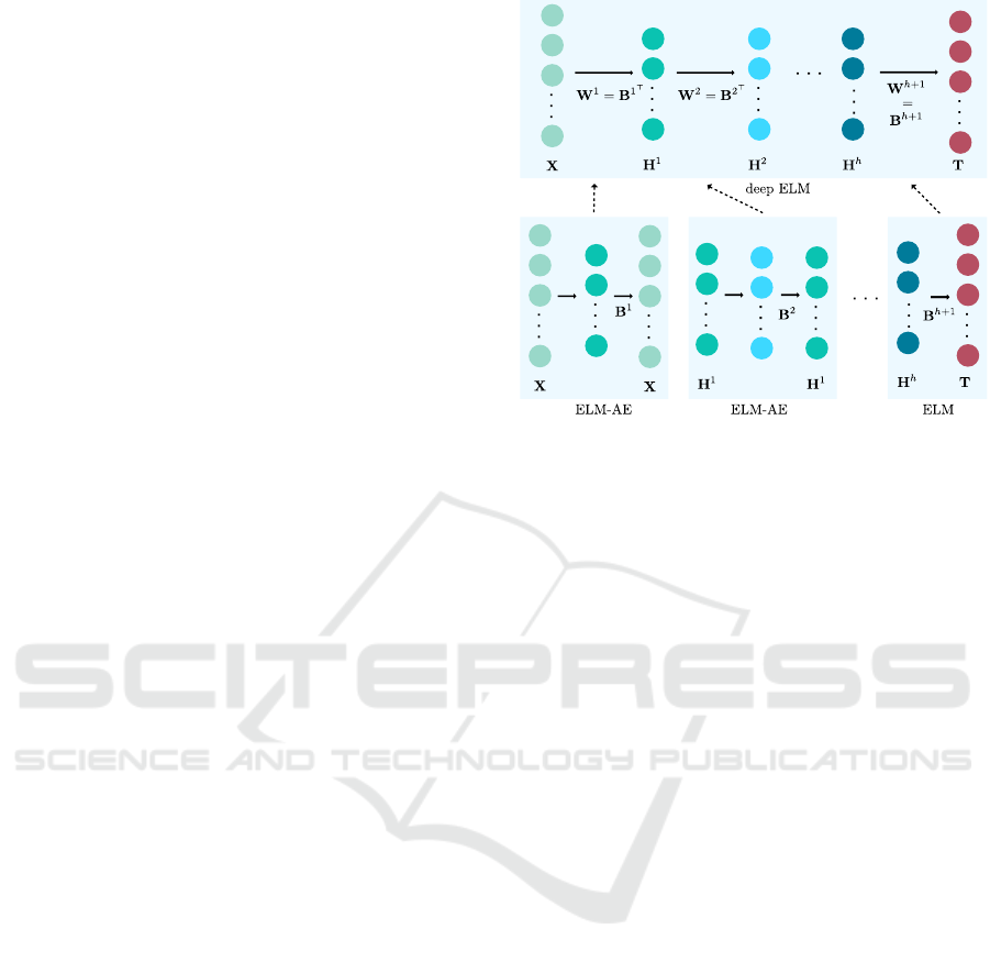
Uzair et al. proposed the use of ELM-based AEs
to construct a deep ELM. It is defined as multiple-
layer neural network whose parameters are learned
by training a cascade of multiple ELM-AE lay-
ers. A fully connected multi-layer network with h
hidden layers is comprised of the parameters L =
{W
1
...W
h+1
}, where W
i
= [w
i
1
...w
i
n
i
]
⊤
∈ R
n
i+1
×n
i
.
Each layer is trained as individual ELM-AE, i.e. the
targets are set the same as the inputs. For exam-
ple, W
1
is learned using the corresponding ELM with
T = X. The weight vectors are initialised orthonor-
mal, as the orthogonalization of these random weights
tends to better preserve pairwise distances in the fea-
ture space (Johnson and Lindenstrauss, 1984) com-
pared to independent random initialisation. Next, de-
pending on the number of hidden layer nodes and
training samples, equation (5) or (7), is used to cal-
culate B
1
. These AE weights re-project the random
representation of the input data back into its origi-
nal space while minimizing the reconstruction error.
Therefore, it is used as the weight matrix of the first
layer W
1
= B
1
⊤
. The weights of the following layers
are learned accordingly by setting the in- and output
of layer h to the representation of the previous layer
H
h−1
. The computation of B with equation (5) or (7)
does not ensure orthogonality. However, orthogonal-
ity results in a more accurate solution since the data
always lie in the same space. Therefore, B is cal-
culated as the solution to the Orthogonal Procrustes
problem
B
∗
= min
B
kHB− Tk
2
, (8)
s.t. B
⊤
B = I.
The closed form solution is obtained by finding the
nearest orthogonal matrix to the given matrix M =
H
⊤
T. To find the orthogonal matrix B
∗
, the singular
value decomposition M = UΣV
⊤
is used to compute
B
∗
= UV
⊤
.
Figure 1 illustrates the training procedure. Note
that the final layer weights a learned as standard ELM
while the lower layers are initialised as ELM-AE.
3.3 Feature Extraction
The openEAR toolkit (Eyben et al., 2009) was used to
extract 6552 features as 39 functionals of 56 acoustic
low-level descriptors and their corresponding first and
second order delta regression coefficients. We applied
the feature extraction on utterance level. Thus, every
utterance, i.e. time series of variable length, is repre-
sented as a single vector of 6552 elements. Details on
Figure 1: Representation learning in deep ELM using ELM-
AE to learn the lower layer weights W
1
to W
h
. The final
layer is trained on the actual target data as standard ELM.
the functionals and acoustic low-level descriptors are
given in (Schuller et al., 2009b). Further, speaker nor-
malisation was carried out by subtraction of the mean
and division by the standard derivation for every fea-
ture and every speaker.
3.4 Experimental Setup
To ensure speaker independence of the classifier the
experiments are carried out in a Leave-One-Speaker-
Out (LOSO) manner. That is, one speaker is left out
for testing, while the remaining speakers are used for
training. This is repeated until every speaker was used
for testing once. The final classification results are
computed as the mean over all runs.
As classes are unbalanced (cf. Table 1), classifiers
are evaluated according to the unweighted average
(UA), and weighted average (WA) of class wise ac-
curacy (Schuller et al., 2009a).
For each database we used single ELM classifiers
to distinguish the six or seven classes. Several hyper-
parameter had to be set, i.e. number of layers h, num-
ber of hidden units n
h
per layer, transfer function f
net
and the tradeoff coefficient C. The experiments to fix
the hyper-parameterswere carried out on EMO-DB. It
is the smallest database and requires the least amount
of time for training.

4 RESULTS
4.1 EMO-DB
Starting with an ELM, where the input weights are
trained as auto-encoder (SL ELM-AE), we tested
different configurations for the activation function
f
net
(x) ∈ {sig(x),tanh(x)} and tradeoff coefficient
C = {10,100,...,10
6
} with n
h
= {50, 100,.. .,3000}.
To check the stability of the classifier each LOSO ex-
periment was repeated 10 times for each parameter
configuration. The reported accuracies are the mean
of these 10 runs.
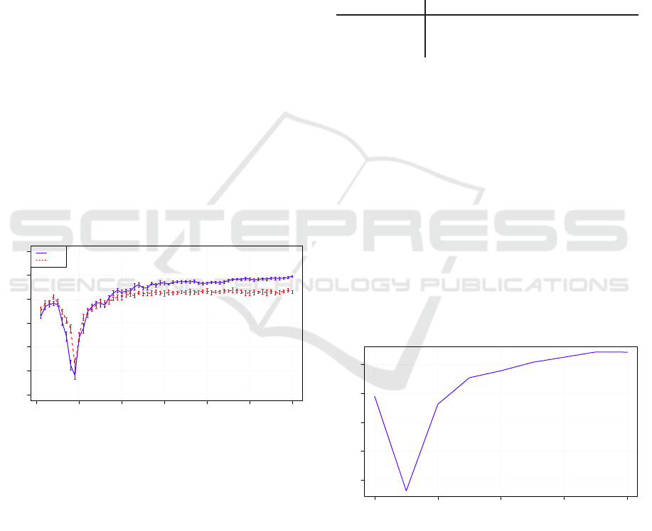
In general, the performance increases with in-
creasing number of hidden nodes, however for all
configurations we observed a performance drop in
the range of n
h
= 250 to 800. For larger n
h
the
performance saturated around WA ≈ 84% in most
cases. Figure 2 shows the results for f
net
(x) ∈
{sig(x),tanh(x)} and C = 100. Besides the drop at
small n
h
one can see, that the interval mean ± stan-
dard deviation gets smaller for larger n
h
. The combi-
nation f
net
(x) = tanh(x) with C = 100 performed best
and did not saturate at n
h
= 3000 with 89.6% WA.
With further increase of n
h
we found the best perform-
ing combination with f
net
(x) = tanh(x), C = 100 and
n
h
= 4100 resulting in 90% WA.
0 500 1000 1500 2000 2500 3000
0.4 0.5 0.6 0.7 0.8 0.9 1.0
n
h
WA
tanh
sig
Figure 2: Weighted average (WA) of class wise accuracy of
SL ELM-AE with C = 100, f
net
(x) ∈ {sig(x), tanh(x)} and
increasing number of hidden nodes n
h
on EMO-DB corpus.
In a follow-up experiment, we used a multi-
layer (ML) ELM, also trained as ELM-AE (cf. Sec.
3.2). We kept C = 100, f
net
(x) = tanh(x) and varied
n
1
h
,n
2
h
= {1000, 1100, . ..,5000}. The performance
did not exceed 84% WA for any of the combinations,
which leads to the conclusion that an additional layer
of abstraction did not support the actual separation
task of different emotional classes.
Finally, we tested a standard ELM with random
input weights and fixed C = 100, f
net
(x) = tanh(x).
Weights were initialised uniformly distributed in the
range (−0.5,0.5). The number of hidden nodes was
increases starting at n
h
= 500 up to 70000 before the
performance saturated at 87.6% WA. Table 2 shows
the best performing configurations for the three tested
approaches, i.e. single-layer (SL) ELM-AE, multi-
layer (ML) ELM-AE, and standard ELM with random
input weights.
Table 2: EMO-DB classification performance of different
ELM approaches with C = 100 and f
net
(x) = tanh(x). We
show mean ± standard deviation of unweighted average
(UA), and weighted average (WA) of class wise accuracy
of 10 runs.
Classifier
n
h
WA UA
SL ELM-AE 4100 90.0±0.4 87.2± 0.6
ML ELM-AE
4000, 4000 84.0± 0.8 82.0± 1.1
ELM
70000 87.6± 0.6 87.0± 0.8
4.2 eNTERFACE
Based on the results on EMO-DB (cf. Table 2), we
kept C = 100, f
net
(x) = tanh(x) fix and varied only
n
h
= {1000,1250,...,3000} to evaluate the SL ELM-
AE performance on the eNTERFACE corpus. The
results are shown in Figure 3. Again, we observed
a drop at lower numbers of hidden units n
h
= 1250
and a saturation starting at n
h
= 2750. For the sake
of training time and computational resources we used
only a single LOSO trail for this evaluation. How-
ever, as this database contains much more utterances
and 43 speakers the variation between different LOSO
trails is small compared to EMO-DB. The best per-
formance was observed at n
h
= 2750 with 74.4% WA
and 74.4% UA.
1000 1500 2000 2500 3000
0.3 0.4 0.5 0.6 0.7
n
h
WA
Figure 3: Weighted average (WA) of class wise accuracy
of a SL ELM-AE with C = 100, f
net
(x) = tanh(x) and in-
creasing number of hidden nodes n
h
on the eNTERFACE
corpus.
4.3 SmartKom
For the SmartKom corpus we evaluated the SL ELM-
AE with C = 100, f
net
(x) = tanh(x) and varied the

number of hidden units n
h
in the range from 50 to
7000
2
. The results are shown in Figure 4. This time
the best performance was observed at a rather low
number of hidden units n
h
= 350 with 53.6% WA and
33.4% UA.
0 1000 2000 3000 4000 5000 6000 7000
0.30 0.35 0.40 0.45 0.50
n
h
WA
Figure 4: Weighted average (WA) of class wise accuracy of
a SL ELM-AE with C = 100, f
net
(x) = tanh(x) and increas-
ing number of hidden nodes n
h
on the SmartKom corpus.
5 DISCUSSION
We applied the representation learning approach in
ELMs as presented in (Uzair et al., 2016) to speech
emotion recognition. To fix the hyper-parameter like
transfer function f
net
and tradeoff coefficient C, sev-
eral experiments were run on the smallest database
EMO-DB. Table 2 summarises these experiments.
Two interesting outcomes could be observed: (i) an
additional layer of abstraction does not support the
actual task to separate the different emotion classes;
(ii) a standard ELM with random input weights per-
forms remarkable well, given a large number of hid-
den nodes. We think these observations show that the
extracted features (cf. Sec. 3.3) already capture a lot
of information for the multi-class problem considered
in this paper. Hence, an extra layer of feature learning
is neither necessary nor helpful.
For the ELM and SL ELM-AE we saw both clas-
sifier to perform very well. While the SL ELM-AE
needed 4100 hidden units, the randomly initialised
ELM reached a comparable high performance with
70000 hidden units (cf. Table 2). Thus, it might be
possible to compensate the drawback of a random
weight initialisation with a sufficiently large amount
of dimensions (hidden units) in the random feature
space.
Given the SL ELM-AE with the highest per-
formance on EMO-DB, we evaluated this setting
on the more challenging corpora eNTERFACE and
SmartKom. As discussed in Section 2, SmartKom
2
n
h
= {50,100,... ,500,750,... ,3000,3500,.. . ,7000}
poses the hardest challenge due to its noisy recod-
ing environment, unbalanced classes and less pro-
nounced, non-acted speech. We cannot pinpoint the
reason for the high performance with a small num-
ber of hidden units n
h
= 350 (cf. Fig. 4) compared to
EMO-DB (n
h
= 4100) and eNTERFACE (n
h
= 2750)
(cf. Figs. 2 and 3).
To rank our results we compare them against the
yet best
3
published results given in (Schuller et al.,
2009b) and (Stuhlsatz et al., 2011). Stuhlsatz et al.
learned discriminative features with Generalized Dis-
criminant Analysis (GerDA) based on deep neural
networks. The GerDA features were used for classi-
fication with a Mahalanobis minimum-distance clas-
sifier. Schuller et al. used SVMs with polynomial
Kernel and pairwise multi-class discrimination based
on Sequential Minimal Optimisation on the same fea-
tures that we used. Table 3 shows the results side by
side.
Table 3: Weighted average (WA) and unweighted average
(UA) class wise accuracy of SVM, GerDA and SL ELM-AE
on acoustic emotion recognition in three different speech
corpora. The best results for each corpus and evaluation
measure are highlighted. SVM and GerDA accuracies were
published in (Stuhlsatz et al., 2011)).
Corpus Classifier
WA UA
EMO-DB
SL ELM-AE 90.0± 0.4 87.2± 0.6
ELM
87.6± 0.4 87.0± 0.8
SVM
85.6 84.6
GerDA
81.9 79.1
eNTERFACE
SL ELM-AE
74.4 74.4
SVM
72.4 72.5
GerDA
61.1 61.1
SmartKom
SL ELM-AE
53.6 33.4
SVM
39.0 23.5
GerDA
59.5 25.0
The SL ELM-AE outperformed the SVM on all
three corpora according to WA and UA. Concern-
ing the GerDA approach, SL ELM-AE yielded the
highest performance on EMO-DB and eNTERFACE
but only achieved 53.6% compared to 59.5% WA
(GerDA) on the SmartKom database.
As GerDA is a data-driven feature learning ap-
proach it benefits from the comparable high amount
of training data in the SmartKom corpus, which sup-
ports the learning of highly compact and discrimina-
tive features (Stuhlsatz et al., 2011). This explains
also the rather weak performance of GerDA on EMO-
DB and eNTERFACE.
In summary our ELM-based approach shows
promising results on all three considerably different
emotional speech databases. It remains to be seen
whether this high performance is stable throughout
3
To our knowledge

other corpora. However, given the simplicity of the
method and the variety of the already tested corpora
we are confident that the ELM/ELM-AE can achieve,
at least, comparable results to the SVM on other
databases as well.
REFERENCES
Bengio, Y., Courville, A., and Vincent, P. (2013). Represen-
tation learning: A review and new perspectives. IEEE
Transactions on Pattern Analysis & Machine Intelli-
gence, 35(8):1798–1828.
Burkhardt, F., Paeschke, A., Rolfes, M., Sendlmeier, W. F.,
and Weiss, B. (2005). A Database of German Emo-
tional Speech. In Proc. Interspeech, pages 1517–
1520.
Eyben, F., W¨ollmer, M., and Schuller, B. (2009). Open-
ear - introducing the munich open-source emotion and
affect recognition toolkit. In 2009 3rd International
Conference on Affective Computing and Intelligent In-
teraction and Workshops, pages 1–6.
Huang, G.-B., Zhou, H., Ding, X., and Zhang, R. (2012).
Extreme Learning Machine for Regression and Mul-
ticlass Classification. IEEE Transactions on Sys-
tems, Man, and Cybernetics, Part B (Cybernetics),
42(2):513–529.
Johnson, W. B. and Lindenstrauss, J. (1984). Extensions of
Lipschitz mappings into a Hilbert space. In Confer-
ence in modern analysis and probability, volume 26,
pages 189–206.
Martin, O., Kotsia, I., Macq, B., and Pitas, I. (2006). The
eNTERFACE’05 Audio-Visual Emotion Database. In
22nd International Conference on Data Engineering
Workshops (ICDEW’06), pages 1–8. IEEE.
Schuller, B., Steidl, S., and Batliner, A. (2009a). The IN-
TERSPEECH 2009 Emotion Challenge. In Proc. In-
terspeech, pages 312–315.
Schuller, B., Steidl, S., Batliner, A., Burkhardt, F., Dev-
illers, L., Christian, M., and Narayanan, S. (2010).
The INTERSPEECH 2010 Paralinguistic Challenge.
In Proc. Interspeech, pages 2794–2797.
Schuller, B., Steidl, S., Batliner, A., N¨oth, E., Vinciarelli,
A., Burkhardt, F., van Son, R., Weninger, F., Eyben,
F., Bocklet, T., Mohammadi, G., and Weiss, B. (2012).
The interspeech 2012 speaker trait challenge. In Proc.
Interspeech, pages 254–257.
Schuller, B., Vlasenko, B., Eyben, F., Rigoll, G., and
Wendemuth, A. (2009b). Acoustic emotion recogni-
tion: A benchmark comparison of performances. In
2009 IEEE Workshop on Automatic Speech Recogni-
tion Understanding, pages 552–557.
Steidl, S. (2009). Automatic Classification of Emotion-
Related User States in Spontaneous Children’s
Speech. PhD thesis, Technische Fakult¨at der Univer-
sit¨at Erlangen-N¨urnberg.
Steininger, S., Rabold, S., Dioubina, O., and Schiel, F.
(2002). Development of the user-state conventions for
the multimodal corpus in smartkom. In Proc. of the
3rd Int. Conf. on Language Resources and Evaluation,
Workshop on Multimodal Resources and Multimodal
Systems Evaluation, pages 33–37.
Stuhlsatz, A., Meyer, C., Eyben, F., Zielke, T., Meier,
G., and Schuller, B. (2011). Deep neural networks
for acoustic emotion recognition: Raising the bench-
marks. In 2011 IEEE International Conference on
Acoustics, Speech and Signal Processing (ICASSP),
pages 5688–5691.
Uzair, M., Shafait, F., Ghanem, B., and Mian, A. (2016).
Representation learning with deep extreme learning
machines for efficient image set classification. Neu-
ral Computing and Applications, pages 1–13.