
Neural Network Inverse Model for Quality Monitoring
Application to a High Quality Lackering Process
Philippe Thomas
1,2
, Marie-Christine Suhner
1,2
, Emmanuel Zimmermann
1,2,3
, Hind Bril El Haouzi
1,2
,
André Thomas
1,2
and Mélanie Noyel
3
1
Université de Lorraine, CRAN, UMR 7039, Campus Sciences, BP 70239, 54506 Vandœuvre-lès-Nancy cedex, France
2
CNRS, CRAN, UMR7039, France
3
Acta-Mobilier, parc d’activité Macherin Auxerre Nord 89270 Moneteau, France
Keywords: Neural Network, Product Quality, Inverse Model, Quality Monitoring.
Abstract: The quality requirement is an important issue for modern companies. Many tools and philosophies have
been proposed to monitor quality, including the seven basic tools or the experimental design. However, high
quality requirement may lead companies to work near their technological limit capabilities. In this case,
classical approaches to monitor quality may be insufficient. That is why on line quality monitoring based on
the neural network prediction model has been proposed. Within this philosophy, the dataset is used in order
to determine the optimal setting considering the operating point and the product routing. An inverse model
approach is proposed here in order to determine directly the optimal setting in order to avoid defects
production. A comparison between the use of a classical multi-inputs multi-outputs NN model and a
sequence of different multi-inputs single-output NN models is performed. The proposed approach is tested
on a real application case.
1 INTRODUCTION
Product quality control is became a major issue in
the mass customization context. Different policies,
such as Total Quality Management (TQM) or Just in
Time (JiT), have been developed in order to control
quality. These two policies are related to the Lean
Manufacturing (LM) concept (Vollmann et al.,
1984).
These policies require the use of different tools,
such as the seven basic quality tools (Ishikawa chart,
check sheet, control charts, histogram, Pareto chart,
scatter diagram, stratification) which allow to
control quality a posteriori. This approach leads to
reject or to downgrade a large part of the production
(Thomas et al., 2013).
A first improvement was given by Taguchi
(1989) which proposed to set up the parameters
control in order to avoid the defects production. The
aim of the Optimal Experimental Design (ODE)
proposed by Taguchi is to provide a setting of the
parameters robust to changing conditions. However,
robust setting is generally non optimal when the
actual conditions are considered. Well, for high
quality production, the process works often near the
limits of its capabilities. In this case, non optimal
setting are insufficient to limit the defects production
(Noyel et al., 2013a).
Noyel et al., (2013b) have proposed to exploit
the production data, collected and stored with
traceability goal, in order to perform on-line quality
monitoring. This approach exploits prediction
models able to predict the defect occurrence risk as a
function of the actual operating range and the
product routing.
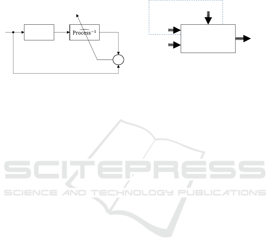
In order to improve this approach, another
philosophy can be exploited. In the domain of
automatic control, adaptive inverse control is based
on inverse processes identification where the output
of the process becomes the input of the model
(figure 1) (Widrow and Bilello, 1993).
The design of the inverse model is often
performed by using the neural network approach and
this type of control has been applied with success to
the control of many non linear process such as,
synchronous motor (Liu et al., 2013), Maglev
system (Hajimani et al., 2014) and robotic (Yildirim,
2004).
The main idea developed here, is to propose an
on line quality monitoring approach based on
Thomas P., Suhner M., Zimmermann E., Bril El Haouzi H., Thomas A. and Noyel M.
Neural Network Inverse Model for Quality Monitoring - Application to a High Quality Lackering Process.
DOI: 10.5220/0006485901860191
In Proceedings of the 9th International Joint Conference on Computational Intelligence (IJCCI 2017), pages 186-191
ISBN: 978-989-758-274-5
Copyright
c
2017 by SCITEPRESS – Science and Technology Publications, Lda. All rights reserved
inverse neural model. The goal is to design a model
able to determine the optimal setting from the
tunable parameters, considering the operating point,
the product routing and the defects occurrence risks.
Process
-
+
error
input
Figure 1: Inverse identification (Widrow and Bilello,
1993).
The main goal of such approach is to obtain
directly a setting able to avoid defects. Moreover, if
a pruning procedure is performed on the neural
model, some inputs may be removed of the model. If
one or more of these inputs correspond to defect
types, this implies that a subsidiary benefit is to
determine if a tunable parameter has an impact or
not on some defect types occurrence.
First we will recall succinctly the quality
monitoring problem. In a second step, the proposed
procedure will be describe. Two approaches will be
discussed:
Using of one multi inputs multi outputs (MIMO)
model;
Using of several multi inputs single output
(MISO) models;
The structure of the neural network and the tools
used will be also presented. After, the industrial
application case and the results obtained will be
presented before to conclude.
2 QUALITY MONITORING
Quality monitoring needs to understand which
factors have an impact on the defects production.
Ishikawa (1986) has proposed the 6M method which
classes these factors into 6 categories: Machine
(technology), Method (process), Material, Man
Power, Measurement (inspection), Milieu
(environment). In the context of on line quality
monitoring which needs to design a prediction
model of the defect, it is more useful to classify
these factors into controllable and non-controllable
factors (Noyel et al., 2013b). The controllable
factors group together the setup parameters when the
non-controllable factors include the operating point
(environmental factors, process constraints…) and
the routing product factors.
Setup
parameters
Environmental
factors
Routing
product
Defects
types
Uncontrollable factors
process
Figure 2: Data collection.
So, in this context, three main types of data must
be collected and stored: controllable and
uncontrollable factors upstream of the process, and
the defects types downstream of the process (figure
2).
Two ways may be used to search the “zero defect”
goal:
By optimizing the settings of various factors;
By drifts monitoring and prevention;
The on line quality monitoring philosophy refers to
the first way. The goal is to determine the best
setting of the controllable factors, for each product
or batch (taking into account its routing constraints),
considering the existing conditions (current
operating point) (Thomas et al., 2013).
3 ON LINE QUALITY
MONITORING
The proposed approach is based on the design of a
neural model able to determine the optimal setting of
controllable factors. The neural network used here is
a multilayer perceptron which seems to be perfectly
adapted to our needs because it is an universal
approximator (Cybenko, 1989, Funahashi, 1989).
3.1 Multilayers Perceptron
The classical multilayer perceptron (MLP) is a
feedforward neural network including only one
hidden layer using a sigmoidal activation function
and on output layer using an activation function
which can be linear for regression problem or
sigmoidal for classification problem. Its structure is
given by (for the output k):
0
1
2101
21
11
2
..
1...
n
n
kkiihhik
ih
zg wg wxb b
with k n
(1)
where,
k
z
are the
2
n
outputs and
0
h
x
are the n
0
inputs
of the neural network,
1
ih
w are the weights
connecting the input layer to the hidden layer,
1
i
b
are
the biases of the hidden neurons,
g
1
(.) is the
activation function of the hidden neurons (here, the
hyperbolic tangent),
2
ki
w
are the weights connecting
the hidden neurons to the output
k,
k
b is the bias of
the output neuron
k, g
2
(.) is the activation function of
the output neuron. Because of the problem is to
obtain the optimal setting of controllable parameters,
we are faced to a regression problem, so
g
2
(.) being
chosen linear.
No normalisation is performed on the dataset.
This fact implies to use an initialisation algorithm
able to take into account the different value ranges
between the inputs (Nguyen and Widrow, 1990).
The dataset is a real industrial dataset polluted
with outliers. So the learning algorithm used must be
robust to these outliers (Thomas et al., 1999). In
order to evaluate the generalization capabilities of
the model, the dataset must be divided into learning
and validation datasets. The learning dataset is used
in order to adapt the parameters of the MLP when
the validation one is used to estimate the
performance of the model.
The accuracy of the neural model depends on the
structure (number of hidden neurons, inputs and
parameters). Too few parameters or hidden neurons,
and the learning can’t find accurate parameters. Too
much parameters, and the learning can lead to the
well-known overfitting problem. To avoid this
problem, the learning is performed on a largely
oversized structure with too much hidden neurons
and a pruning procedure is used to reduce this
structure (Thomas and Suhner, 2015). This
procedure presents the advantage to be able to
discard some spurious inputs.
3.2 Tuning of Controllable Parameters
The main idea is to determine the optimal setting of
the controllable parameters by using MLP model.
This model is designed by using the dataset
constituted by the controllable and uncontrollable
factors collected upstream of the process, and the
defects types collected downstream of the process.
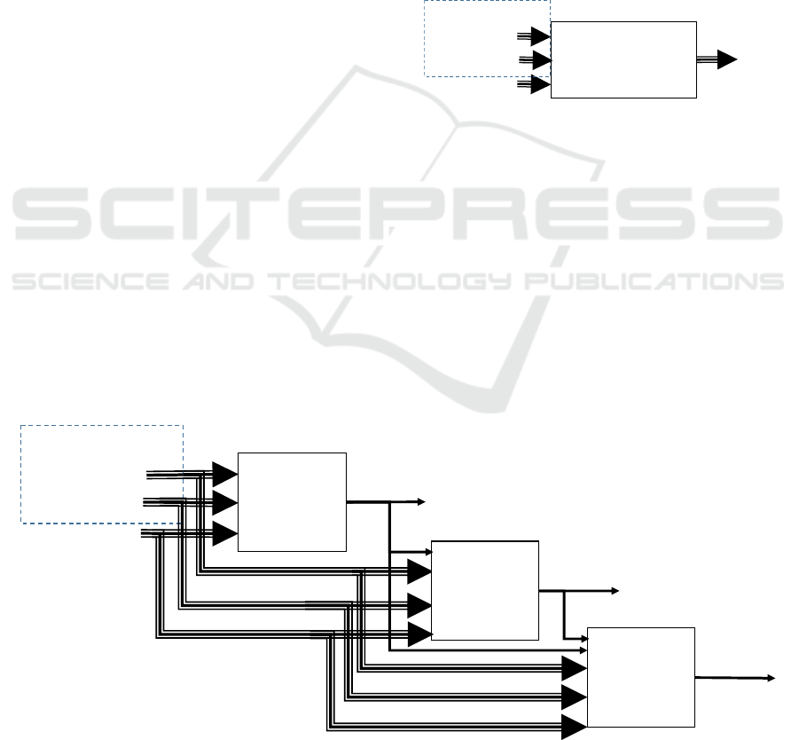
This model is designed under the inverse concept
where the outputs of the model are constituted by
some inputs of the process, when the inputs of the
models includes some inputs of the process and its
outputs (figure 3).
Setup
parameters
Environmental
factors
Routing
product
Defects
types
Uncontrollable factors
NN model
Figure 3: Inverse model design.
To do that, the classical and simplest approach is
to design a multi-inputs multi-outputs (MIMO)
neural network. However, in this case, the pruning
phase don’t allow to determine if a defect type
(input) is related to a particular setup parameter
(output).
To outperform this drawback, another structure
is used, where different multi-inputs single-output
(MISO) neural networks are designed sequentially.
The figure 4 presents an example of such structure,
where 3 setup parameters are considered.
Setup
Parameter 1
Environmental
factors
Routing
product
Defects
types
Uncontrollable factors
NN MISO
model 1
NN MISO
model 2
Setup
Parameter 2
NN MISO
model 3
Setup
Parameter 3
Figure 4: Sequential MISO NN models (case of 3 setup parameters).

Considering this structure, four advantages can
be listed:
Each NN model includes less parameters (only
one output, possibly less hidden neurons,
possibly more inputs pruned). This fact improves
the learning and using speeds and limits the
overfitting risk.
The learning of each NN model is independent.
This fact implies that the learning of these
different model may be performed in parallel.
The pruning step allows to pruned inputs in each
NN model. This fact implies that a causal link
may be discarded between some defect types
(pruned inputs) and the considered setup
parameter.
Each NN model may use, as inputs, the outputs
(setup parameters) of the upstream NN models in
the sequential structure. This fact allows to
improve the global accuracy of the structure.
The sequence of the different MISO NN models
selected is the one which optimize the accuracy of
the complete structure on the validation dataset.
In the sequel, the performances of the proposed
structure will be tested and compared with those
obtained with a single MIMO model on a real
industrial case.
4 INDUSTRIAL APPLICATION
4.1 Presentation of the Process
The considered problem is a quality monitoring
problem in a company which produces high quality
lacquered panels made in MDF (Medium Density
Fibreboard) for kitchen, bathroom, offices, hotel
furniture, stands, shops... This study focuses on its
main process which is a robotic lacquering
workstation. This workstation is free of human
factors, but defects rates are important and very
fluctuant, and could expand from 10% to 45% from
one day to another. This fact is mainly due to the
high quality requirements, which implies that this
workstation works at its limit capabilities. So,
despite the design of an ODE in order to tune this
robotic workstation, the company fails to reduce the
defects rates.
That’s why an on line quality monitoring
approach is performed. Expert knowledge has
allowed to list parameters able to have impact on the
defects generations. These parameters can be
classified into:
Three environmental factors (temperature,
humidity, pressure).
Five product routing parameters (number of
passes, time per table, litre per table, number of
layers, drying time)
Three setup parameters (load factor, basis
weight, number of products).
These different factors and parameters are able to
have an impact on thirty different defects types.
Considering the inverse model structure, the
dataset is constituted by three outputs (setup
parameters) and thirty eight inputs (environmental
factors, product routing parameters, and types of
defects). The dataset includes 2167 data and is split
into two datasets for identification (1088 data) and
validation (1079).
In order to limit the risk of local optimum
trapping, the learning of all the NN models is
performed with twenty initial parameters sets and
the best one is retained.
The selection criterion used is the classical Root
Mean Square Error (RMSE) calculated on the
learning and validation datasets:
2
1
1
() ()
N
n
RMSE z n y n
N
(2)
where
z(n) is the output given by the network for the
data n and y(n) is the corresponding target.
The first NN model designed is the MIMO one.
The initial number of hidden neuron is set to twenty.
Table 1 presents the RMSE values obtained with the
best MIMO model for the three different outputs.
These values highlight the difference between the
variation ranges and amplitudes of the outputs. This
fact may have an impact on the learning accuracy.
During the learning, the criterion to minimize is the
errors sum squared performed on the three outputs.
In this case, the risk is that the learning algorithm
favours one output over the others.
Table 1: RMSE values for the MIMO NN model.
learning validation
load factor 0.4057 0.4406
basis weight 191.8222 238.2346
products number 307.3382 381.0269
The results obtained with the MIMO model must
be compared to those obtained with the sequence of
MISO models.
To design the sequence of MISO models, it is
necessary to determine in which order the setup
parameters must be considered. The selected order is
the one which maximize the sequence accuracy.
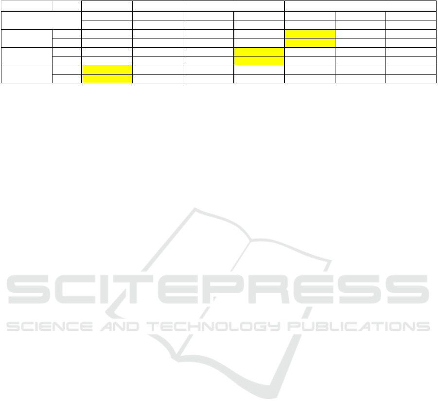
Table 2: RMSE values for the different MISO NN models.
1
st
MISO model
load facto
r
b
asis wei
g
ht
p
roducts number
b
asis wei
g
ht load facto
r
load facto
r
products number products number basis weight
learnin
g
0.3698 0.3509 0.2339 0.2381
validation 0.4336 0.4466 0.2856 0.2805
learning 177.3311 185.1477 182.785 178.9352
validation 230.4716 226.6402 224.0547 228.0947
learning 297.5479 223.1687 365.6229 218.7272
validation 361.2214 264.4579 369.2758 256.713
3
rd
MISO model
supplementary
in
p
uts
Load factor
basis weight
products number
2
nd
MISO model
Different MISO NN models must be designed
with different structures. For all these models the
initial number of hidden nodes is setup to twenty.
The inputs number depends of the order of the
sequence. The first MISO model must determine its
output by using the same thirty eight inputs of the
MIMO model. The second one shall have one
additional input (the output of the first MISO
model). The third one shall have two additional
inputs (the outputs of the two preceding MISO
models).
The table 2 presents the RMSE values obtained
for the learning and the validation datasets for the
different MISO NN models designed. The first line
indicates if the considered model is the first, the
second or the third of the sequence. The second line
indicates which the supplementary inputs if
available are.
First, it can be noticed that the use of one or two
supplementary inputs improve the accuracy for the
three outputs. As example, the RMSE value for the
validation dataset for load factor is reduced with a
reduction from 0.4336 to 0.2856 (34%
improvement) when product number is used as
supplementary input. The same observation may be
performed for the two other outputs.
So it is necessary to determine the optimal
sequence of MISO models. To do that, the decrease
in terms of percent of RMSE (compared with the
results obtained with the MIMO model) is studied
and the sequence which minimizes the sum of the
three “RMSE decreased in terms of percent” values
for the three outputs (on the validation dataset) is
selected. With this criterion, two sequences gives
very similar results:
First: products number (5%); second: basis
weight (6%); third: load factor (36%).
First: products number (5%); second: load factor
(35%); third: basis weight (4%).
For the sequel, we choose arbitrarily the first
sequence and the results obtained for the three
MISO models of the sequence are highlighted in
table 2. This is these results which must be
compared to those obtained with the MIMO models
presented table 1. These results show a slight
improvement for two outputs (5% for products
number and 6% for basis weight) which is not very
significant. However, the improvement obtained for
the third output (load factor) is relevant and reaches
36%.
It can be noticed that the choice of the sequence
is important to obtain the best results, but all
sequences allows to improve substantially the results
compared to those obtained with the MIMO model.
In our case, the worst sequence is:
First: load factor (2%);
Second: products number (4%);
Third: basis weight (31%).
The choice of the sequence may also be performed
by using expert knowledge.
The three selected MISO models have been
pruned in order to find the optimal structure of the
model and to limit the overfitting risk. A second
advantage is, that it allows to determine if a causal
link occurs between the considered setup parameter
(output) and the defects types (some of the inputs).
For the setup parameter “products number” the
pruning algorithm has preserved only one defect
type: “grain on face”. This fact implies that the
optimal tuning of this parameter has no impact on
the twenty nine other defects types.
For the second setup parameter: “basis weight”,
only three defects types are discarded: “grain on
back”, “scratch” and “sanding defect”. So, the
optimal setting of this parameter may have an
impact on the twenty seven other defects types.
For the third setup parameter: “load factor”,
seven defects types are discarded: “grain on back”,
“stain under the paint”; “scratch”, “paint refusal”;
“priming defect”, “sanding defect”, “silicone mark”.
It can be noticed that some types of defects are
impacted by none of the setup parameters: “grain on
back”, “scratch” and “sanding defect”. This is due to
the fact that these types of defects don’t find their
origin in the considered workstation. Scratch defects
are mainly caused by handling problem. Sanding
defect are certainly produced during the preceding
sanding step. Grain on back are performed during a

preceding step of lacquering.
It can be noticed that some defects types which
probably don’t find their origin in the considered
workstation are not pruned in the second MISO
model: “priming defect” or “silicone mark”. This
fact is probably due to the pruning algorithm
accuracy.
5 CONCLUSIONS
An on line quality monitoring approach based on
neural network models is proposed here. The main
goal of this proposed approach is to determine
quickly and simply the optimal tuning of setup
parameters considering the actual operating point
and the product routing. This quality monitoring is
based on inverse approach NN models which try to
determine the tuning of setup parameters by using
both, non controllable parameters collected upstream
of the workstation, and quality defects occurrence
collected downstream of the workstation.
Two approaches may be used to perform the
design of the inverse model. The simplest is to use a
multi-inputs multi-outputs model able to set up all
the controllable parameters simultaneously. The
second one is to use a sequence of different multi-
inputs single-output models able each to set up only
one parameter. These two approaches are tested and
compared. The results have shown that the second
approach allows to improve the accuracy of the
complete system.
Moreover, the using of a pruning algorithm next
the learning allows to determine if a causal link
occurs between some defects types and the
considered setup parameter.
In some extreme environmental conditions, it is
possible that none setup is able to avoid defects
production for certain product routing. In this case,
one drawback of the proposed approach is that our
system will give a setup, possibly the best one, but
which will be insufficient. Our future works will
focus on the detection of these particular conditions
in order to be able to propose to the operator to delay
the machining of the considered products.
REFERENCES
Cybenko, G., 1989. Approximation by superposition of a
sigmoïdal function. Math. Control Systems Signals, 2,
4, 303-314.
Hajimani, M., Dashti, Z.A.S., Gholami, M., Jafari, M.,
Shoorehdeli, M.A., 2014. Neural adaptive controller
for magnetic levitation system, Iranian Conf. on
Intelligent Systems ICIS’14, Bam, Iran.
Ishikawa, K., 1986. Guide to quality control. Asian
Productivity Organization.
Liu, G.,Chen, L., Zhao, W., Jiang, Y., Qu, L., 2013.
Internal Model control of permanent Magnet
synchronous motor using support vector machine
generalized inverse, IEEE Trans. on Industrial
Informatics, 9, 2, 890-898.
Nguyen, D., Widrow, B., 1990. Improving the learning
speed of 2-layer neural networks by choosing initial
values of the adaptative weights. Proc. of the Int. Joint
Conference on Neural Networks IJCNN'90, 3, 21-26.
Noyel, M., Thomas, P., Charpentier, P., Thomas, A.,
Brault, T., 2013a. Implantation of an on-line quality
process monitoring. 5
th
Int. Conf. on Industrial
Engineering and Systems Management IESM'13a,
Rabat, Maroc.
Noyel, M., Thomas, P., Charpentier, P., Thomas, A.,
Beauprêtre, B., 2013b. Improving production process
performance thanks to neuronal analysis. 11
th
IFAC
Workshop on Intelligent Manufacturing Systems
IMS'13, Sao Paulo, Brazil.
Taguchi, G., 1989. Quality enginnering in production
systems, NY, MacGraw-Hill.
Thomas, P., Bloch, G., Sirou, F., Eustache, V., 1999.
Neural modeling of an induction furnace using robust
learning criteria. J. of Integrated Computer Aided
Engineering, 6, 1, 5-23.
Thomas, P., Noyel, M., Suhner, M.C., Charpentier, P. and
Thomas, A., 2013. Neural Networks ensemble for
quality monitoring, 5
th
Int. Joint Conf. on
Computational Intelligence IJCCI'13, Vilamoura,
Portugal, 515-522.
Thomas, P., Suhner, M.C., 2015. A new multilayer
perceptron pruning algorithm for classification and
regression applications. Neural Processing Letters, 42,
2, 437-458
Vollmann, T.E., Berry, W.L. and Whybark, C.D., 1984.
Manufacturing Planning and Control Systems, Dow
Jones-Irwin.
Widrow, B., Bilello, M., 1993. Adaptive inverse control,
Proc. of the Int. Symp. on Intelligent Control, Chicago,
Illinois, USA.
Yildirim, S., 2004. Adaptive robust neural controller for
robots. Robotics and Autonomous Systems, 46, 3, 175-
184.
