
Ant Colony Optimization Approaches for the Tree t-Spanner Problem
Manisha Israni and Shyam Sundar
Department of Computer Applications, National Institute of Technology Raipur, Raipur (Chhattisgarh), India
Keywords:
Tree Spanner, Weighted Graph, Swarm Intelligence, Ant Colony Optimization.
Abstract:
A tree t-spanner of a given connected graph is a spanning tree T in which the ratio of distance between every
pair of vertices is at most t times their distance in the graph, where t is a parameter known as stretch factor
of T . The tree t-spanner problem deals with finding a spanning tree in a connected graph whose stretch
factor is minimum amongst all spanning trees of the graph. For unweighted graph, this problem is N P-Hard
for any fixed t ≥ 4, whereas for weighted graph, this problem is N P -Hard for any fixed t > 1. This paper
concerns this problem for connected, undirected, and weighted graph and proposes three variants of ant colony
optimization (ACO) approach for this problem. ACO approach is a swarm intelligence technique inspired by
the foraging behavior of real ants. All three variants of ACO approach have been tested on a set of randomly
generated graph instances. Computational results show the effectiveness of all three variants of ACO approach.
1 INTRODUCTION
Given a connected graph G(V, E), a tree t-spanner is
a spanning tree (say T ) in which the distance between
every two vertices (say u and v) in T is at most t times
their distance in G. t is a parameter called stretch fac-
tor of T and it is determined by the maximum stretch
taken over all pairs of vertices in G, where the stretch
of a pair of vertices (say u and v) in T is the ratio of
the distance between u and v in T to their distance in
G. The tree t-spanner problem aims to find a span-
ning tree of G whose stretch factor (t) is minimum
amongst all spanning trees of G.
The term t-spanner of a graph G, which was first
coined by Peleg and Ullman (Emek and Peleg, 2008),
is a spanning subgraph (H) of G in which the dis-
tance between every pair of vertices is at most t times
their distance in G. This notion (spanner) describes an
property about the approximation of pairwise vertex-
to-vertex distances in the original graph by spanning
subgraph (H). This approximation distance quality is
measured by the parameter t ≥ 1, which is referred to
as the stretch factor of the t-spanner. Spanners with
such distance approximation property make them of
practical relevances in various areas such as commu-
nication networks, distributed systems, motion plan-
ning, network design, and parallel machine architec-
tures (Alth
´
ofer et al., 1993; Awerbuch et al., 1992;
Bhatt et al., 1986; Liestman and Shermer, 1993; Pe-
leg and Ullman, 1987; Peleg and Upfal, 1988). For
example, spanners can be used to build synchronizers
for transforming synchronous algorithms into asyn-
chronous ones (Emek and Peleg, 2008).
In a connected graph, if a spanning subgraph (say
T ) is both t-spanner and tree, then T is referred to
as a tree t-spanner. Note that a spanning tree of the
graph is always a tree spanner, where a tree spanner
is a tree t-spanner for some t ≥ 1. Tree spanners also
find practical relevance. For example, tree spanners
of small stretch factors can be applied in performing
multi-source broadcast in a network (Awerbuch et al.,
1992), which can greatly simplify the message rout-
ing at the cost of only small delay in message delivery.
Later, Cai and Corneil (Cai and Corneil, 1995) stud-
ied graph theoretic, algorithmic, and complexity is-
sues about tree spanners of weighted and unweighted
connected graphs. They proved on edge-weighted
graphs that a tree 1-spanner, if it exists, is a mini-
mum spanning tree and can be found in polynomial
time. They also proved on edge-weighted graphs that
the problem of finding a tree t-spanner is N P -Hard
for any fixed t > 1. In case of unweighted graphs,
the problem of finding a tree t-spanner is N P -Hard
for any fixed integer t ≥ 4. For connected, undi-
rected and unweighted graph, this problem is referred
to as minimum max-stretch spanning tree problem
(Emek and Peleg, 2008; Dragan and K
¨
ohler, 2014).
In literature, approximation algorithms on some spe-
cific types of unweighted graph (Cai, 1992; Peleg and
Tendler, 2001; Venkatesan et al., 1997) have been de-
veloped for the tree t-spanner problem; however, such
specific types of graph may not be encountered in ev-
Israni M. and Sundar S.
Ant Colony Optimization Approaches for the Tree t-Spanner Problem.
DOI: 10.5220/0006490002000206
In Proceedings of the 9th International Joint Conference on Computational Intelligence (IJCCI 2017), pages 200-206
ISBN: 978-989-758-274-5
Copyright
c
2017 by SCITEPRESS – Science and Technology Publications, Lda. All rights reserved

ery situation. One can find various related tree span-
ner problems in details in (Liebchen and W
¨
unsch,
2008).
This paper concerns the tree t-spanner problem
for connected, undirected and edge-weighted graph
G(V, E, w), where V is a set of vertices; E is a set
of edges; and for each edge, there exists an edge
weight which is a positive rational number. Here-
after, the tree t-spanner problem for connected, undi-
rected and edge-weighted graph G(V, E, w) will be re-
ferred to as [Tree] t-SP. Since [Tree] t-SP is N P -
Hard for t > 1, metaheuristic techniques are the ap-
propriate approaches that can find high quality solu-
tion in a reasonable time. In literature, only genetic al-
gorithm (GA) (Moharam and Morsy, 2017) has been
proposed so far for the [Tree] t-SP. GA (Moharam
and Morsy, 2017) is based on generational population
model which uses multi-point crossover and mutation
genetic operators for generating offsprings.
Ant colony optimization (ACO) approach (Dorigo
et al., 1991; Dorigo and St
¨
utzle, 2004) is swarm-
based metaheuristic technique that has been ap-
plied successfully to many combinatorial optimiza-
tion problems. It is inspired by the foraging behavior
of ants. This paper proposes three variants of ACO
approach for the [Tree] t-SP. The proposed three vari-
ants of ACO approach have been tested on a set of
randomly generated graph instances (see description
Section 4.1). On a set of randomly generated graph
instances, computational results show the effective-
ness of the proposed three variants of ACO approach
for this problem.
The rest of this paper is organized as follows: Sec-
tion 2 and 3, respectively, describes a brief introduc-
tion of ACO approach and presents three variants of
ACO approach for the [Tree] t-SP. Computational re-
sults are reported in Section 4. Finally, Section 5 con-
tains some concluding remarks.
2 ACO APPROACH
Ant colony optimization (ACO) approach is a swarm-
based metaheuristic technique derived from the ob-
servation of real ants’ foraging behavior. In nature,
ants wander randomly in search of food and deposit
a chemical substance called pheromones on the paths
while wandering. Other ants can smell pheromones
and tend to choose their way probabilistically based
on paths marked by strong pheromone concentrations,
resulting a pheromone-trail. Pheromones on the paths
also evaporate with time. While returning to the nest
from the food source, ants tend to choose the short-
est path marked by strong pheromone concentrations
in comparison to longer paths, resulting in further in-
crement on pheromone concentrations on such short-
est path. Such strong pheromone trail on this short-
est path stimulates more and more ants to follow
this shortest path again, which in turn, further rein-
forces the pheromone trail on this shortest path. Af-
ter some time, the whole ants in the colony follow
that pheromone trail which leads to the shortest path
from nest to food source and vice versa. Hence such
behavior for searching the shortest path between nest
and food source emerges from the cooperation among
individuals of the whole colony.
This feature of real ant colonies has been emulated
in ant colony optimization (ACO) approach for the so-
lution of hard combinatorial optimization problems.
In ACO approach, each artificial ant in the colony
builds a solution through incremental procedure that
takes the help of heuristic information of the prob-
lem under consideration and pheromone trails that are
accumulated through search experience. Dorigo et
al. (Dorigo et al., 1991) developed the first ACO ap-
proach called Ant System. Later, different variants of
ACO have been proposed in the literature. One can
find a good survey of different variants of ACO algo-
rithms and their applications in (Dorigo and St
¨
utzle,
2004). Readers can find some recent work on ACO
approach (Sundar and Singh, 2013; Sundar et al.,
2012; Monteiro et al., 2015)
3 THREE VARIANTS OF ACO
APPROACH FOR THE [Tree] t-SP
This section presents three variants of ACO approach
for the [Tree] t-SP. All components of each variant of
ACO approach are the same except the updating rule
regarding the pheromone trails component.
Initially, all pairs of shortest paths for a given
graph is precomputed. Also, pheromone value at each
edge of G is initialized with a high value (here the
value is set to 10 which is determined empirically) so
that ACO approach performs a wider exploration of
the search space during initial iterations before start-
ing biasing the search. Then, at every iteration, each
artificial ant in the colony constructs a spanning tree
and computes the fitness of its constructed solution;
and the update of pheromone trails is performed.
3.1 Construction of Solution
Each artificial ant, say k, constructs a spanning tree
(solution), say T , on G(V, E, w) with the help of
heuristic information and pheromone value. Initially,

T is an empty set (Φ). S is another set which is ini-
tially empty (Φ). A vertex, also called root vertex (say
r) of T to be grown, is selected randomly from V and
is added to S. For each vertex x in V , the attribute
d
T
(r, x) that is the distance from the root r of T to x is
maintained. For the root vertex r, d
T
(r, r) is set to 0.
Hereafter, similar to Prim’s algorithm (Prim, 1957),
iteratively, ant k, at each step, selects an edge con-
necting a vertex, say u, in S to a vertex, say v, in V \S;
however, instead of selecting an edge with minimum
cost, an edge is selected according to a probabilis-
tic action choice rule based on heuristic information
and pheromone values. The probability of selecting
an edge (prob
k
e
uv
) by ant k is determined as follows:
prob
k
e
uv
=
[τ
e
uv
]
α
[η
e
uv
]
β
∑
v
1
∈S
∑
v
2
∈V \S
[τ
e
v
1
v
2
]
α
[η
e
v
1
v
2
]
β
(1)
where τ
e
v
1
v
2
is the pheromone concentration on the
edge e
v
1
v
2
; η
e
v
1
v
2
is the heuristic value that is avail-
able a priori, and that is equal to the weight on edge
e
v
1
v
2
; and α and β are two parameters which deter-
mine the relative influence of the pheromone trail and
the heuristic information respectively. By this prob-
abilistic action choice rule, the probability of select-
ing a particular edge (u, v) increases with the value
of associated pheromone trail τ
e
uv
and of the heuris-
tic information value η
e
uv
. The parameters α and β
together help in searching high quality solution in the
search space. Hence, being biased by higher heuristic
and pheromone value, this probabilistic action choice
rule plays an important role in exploring various good
(in terms of fitness) spanning trees in the search space
on a graph instance. The selected edge e
uv
is added
to T and v is added to S. Update d
T
(r, v) through
“d
T
(r, v) = d
T
(r, u) + w(u, v)”. This process is re-
peated until V \S becomes empty. At this juncture,
a spanning tree T is constructed.
3.2 Fitness Computation
Once the spanning tree T that is also a tree spanner
is constructed, its fitness, in terms of its stretch fac-
tor t, is computed. Before computing fitness, lowest
common ancestors for pairs of vertices in T with the
root vertex r, are preprocessed by least common an-
cestor algorithm (Harel and Tarjan, 1984), where low-
est common ancestor for any two vertices, say u and
v, in T is the common ancestor of vertices u and v
that is located farthest from the root, and is referred
to as LCA(u,v). In doing so, one can get the lowest
common ancestor query for any pair of vertices say u
and v in T , i.e., LCA(u, v) in constant-time. Distance
d
T
(u, v) between any two vertices u and v in T can be
computed as
d
T
(u, v) = d
T
(r, u) + d
T
(r, v) − 2 × (d
T
(r, LCA(u, v)))
(2)
One can easily determine the maximum stretch factor
t of T taken over all pairs of vertices x, y in G, i.e.,
d
T
(u, v)
d
G
(u, v)
∀(u, v) ∈ G (3)
3.3 Update of Pheromone Trails
Once all ants have constructed their solutions at
the current iteration (say it) of ACO approach, the
pheromone trails are updated at the end of the cur-
rent iteration, i.e. it. We follow three ways
for the update of pheromone trails based on local
pheromone update, global pheromone update, and
mixed pheromone update that also define three vari-
ants of ACO approach for the [Tree] t-SP.
Local Pheromone Update: First, decrease the
pheromone value on each edge, say e
uv
, of G by a
constant factor, and then augment the pheromone
on those edges of G that are selected by the itera-
tion’s best solution (S
ib
) or that are selected by the
iteration’s best ant. The pheromone trails which
are updated by the iteration’s best ant on the edges
of G are as follows:
τ
e
uv
(it + 1) = ρ τ
e
uv
(it) + ∆τ
ib
e
uv
(4)
where 0 < ρ ≤ 1 is the persistence rate, and ∆τ
ib
v
is
the amount of pheromone that the iteration’s best
ant deposits on the edges of the iteration’s best so-
lution (S
ib
). The parameter ρ is used to avoid un-
limited accumulation of pheromone trails as the
ACO approach progresses, and simultaneously it
also helps the ACO approach in forgetting bad de-
cisions taken in past. In addition, if an edge is not
selected by the ants, the pheromone value of this
edge decreases exponentially in the number of it-
erations. ∆τ
ib
e
uv
is defined as follows:
∆τ
ib
e
uv
=
(
p
aug1
, if e
uv
∈ S
ib
;
0, otherwise.
(5)
where p
aug1
is a parameter to be determined
empirically. This equation explains that the better
the solution S
ib
in terms of fitness is, the more
pheromone the edges that are part of this solution
receive. Hence edges that are part of solution with
higher fitness are more likely to be selected by
ants in future iterations of the approach, thereby
receiving more reinforcement. Hereafter, this

variant of ACO approach will be referred to as
ACO Local.
Global Pheromone Update: It is similar to
local pheromone update except augmenting
pheromone. In this variant of ACO approach,
augment pheromone on those edges of G that
are present in the best-so-far solution (say S
gb
)
found by best-so-far ant since the start of ACO ap-
proach. The pheromone trails which are updated
by the best-so-far ant on the edges of G are as fol-
lows:
τ
e
uv
(it + 1) = ρ τ
e
uv
(it) + ∆τ
gb
e
uv
(6)
where ∆τ
gb
v
is the amount of pheromone best-so-
far ant deposit on the edges of best-so-far solution
(S
gb
). ∆τ
gb
e
uv
is defined as follows:
∆τ
gb
e
uv
=
(
p
aug2
, if e
uv
∈ S
gb
;
0, otherwise.
(7)
where p
aug2
is a parameter to be determined
empirically. Hereafter, this variant of ACO
approach will be referred to as ACO Global.
Mixed Pheromone Update: It is similar to lo-
cal pheromone update except augmenting the
pheromone. In this variant of ACO approach,
two ways in mixed way are applied in augment-
ing the pheromone: first augment the pheromone
on those edges of G that are present in the iter-
ation’s best solution (S
ib
) or that are selected by
iteration’s best ant; and second, at every P
gb
gen-
erations, augment the pheromone on those edges
of G that are present in the best-so-far solution
(say S
gb
) found by best-so-far ant since the start of
ACO approach, where P
gb
is a parameter to be de-
termined empirically. The update of pheromone
trails in this approach is as follows:
τ
e
uv
(it + 1) = ρ τ
e
uv
(it) + ∆τ
mixed
(8)
where ∆τ
mixed
is the sum of amount of pheromone
( ∆τ
ib
e
uv
, i.e. p
aug1
) augmenting on the edges of S
ib
and amount of pheromone (∆τ
gb
e
uv
, i.e. p
aug1
) aug-
menting on the edges of S
gb
at every iter, where
∆τ
ib
e
uv
is similar to equation 5 and ∆τ
gb
e
uv
, which
is applied at every P
gb
generations, is similar to
equation 7. Note that here ∆τ
gb
e
uv
at every P
gb
gen-
erations is additional reinforcement. Hereafter,
this variant of ACO approach will be referred to
as ACO Mixed.
Algorithm 1: Pseudo-code of ACO approach for the
[Tree] t-SP.
Compute all pairs of shortest paths of G;
Initialize pheromone value at each edge of G;
while Termination criteria is not satisfied do
for k ← 1 to pop
ant
do
Each ant k constructs a spanning tree of
G with the help of heuristic information
and pheromone value;
Perform update of pheromone trails;
The lower pheromone trail limit, i.e. τ
min
is ex-
plicitly set for the proposed three variants of ACO ap-
proach. The pseudo-code of ACO approach for the
[Tree] t-SP is given by Algorithm 1, where pop
ant
is
the size of colony (population) of ants.
4 COMPUTATIONAL RESULTS
The proposed three variants of ACO approach
(ACO Local, ACO Global, and ACO Mixed) for the
[Tree] t-SP have been implemented in C and tested
on a set of randomly generated graph instances. All
experiments have been performed on a Linux with the
configuration of 3.2 GHz × 4 Intel Core i5 processor
with 4 GB RAM. Each variant of ACO approach has
been executed 10 independent runs on each instance.
We have allowed each variant of ACO approach to
execute for 1000 generations.
Subsequent subsections discuss about the genera-
tion of graph instances and the parameter tuning. In
addition, a comparison study of all three variants of
ACO approach on graph instances is also discussed.
4.1 Graph Instances
Since instances used in GA (Moharam and Morsy,
2017) for the [Tree] t-SP are not available, and it
should be also noted that authors (Moharam and
Morsy, 2017) tested the effectiveness of their GA on
only two instances (i.e. first instance is a graph of
50 vertices and second one is a graph of 100 ver-
tices (one can see Table 5 of (Moharam and Morsy,
2017)). To test our proposed ACO approaches, two
set of graph instances G(V, E, w) with V = 50, 100 are
generated randomly in 500 × 500 plane. A graph in-
stance is generated as follows: each point represent-
ing a vertex in G is selected randomly in 500 × 500
plane. The Euclidean distance between two vertices
(v
1
, v
2
) is its edge weight. For each set, three different
complete graph instances are generated, and with the
help of each generated graph G
i
(V
i
, E
i
), further three
sparse graphs with different edge density, i.e., |E
i1
|,
|E
i2
|, |E
i3
| are generated, where |E
i1
| = 0.8 × |E
i
|;
|E
i2
| = 0.6 × |E
i
|; and |E
i3
| = 0.4 × |E
i
|. Note that
0.8 × |E
i
| (0.6 ×|E
i
| and 0.4 × |E
i
|) means 20% (40%
and 60%) random edges of E
i
are not considered into
E
i1
(E
i2
and E
i3
). All graph instances are represented
in A1 A2 A3 (see Table 2, where A1 is the total num-
ber of vertices of that graph (see column Vertex of Ta-
ble 2); A2 is X % (see column Edge of Table 2) ran-
dom edges of total number of edges in its correspond-
ing complete graph with A1 vertices are not consid-
ered in current graph instance; and A3 presents dif-
ferent graph instance (in terms of edge density) with
the same number of vertices (A1). In Table 2, con-
sider 50 0.0 1 instance which is a complete graph
with A1 = 50, A2 = 0.0 and A3 = 1. Three different
instances with different edge-density have been gen-
erated from this graph by doing changes in A2, i.e.
A2 = {0.2, 0.4, 0.6}. The generated graph instances
corresponding to 50 0.0 1 are 50 0.2 1, 50 0.4 1 and
50 0.6 1.
Hence, 24 graph instances have been generated
from the two sets of graph instances with |V | ∈ {50,
100}.
Table 1: Possible values of each parameter used in ACO
approaches for the [Tree] t-SP.
Parameter Description Characteristics
ant pop The population of ants {10, 20, 30, 40}
τ
min
Value of τ
min
{0.001, 0.05, 0.01, 0.005}
α A parameter {0, 1, 2}
β A parameter {0, 1, 2}
P A parameter {0.05, 0.1,0.2}
ρ A parameter {0.975, 0.98, 0.985, 0.99}
P
gb
A parameter {10, 20, 30}
4.2 Parameter Tuning
ACO approaches are stochastic approaches, and pa-
rameters used in our proposed three variants of ACO
approach for the [Tree] t-SP play significant roles in
finding high quality solutions. It is to be noted that de-
termining a perfect tuning of various parameters used
is a difficult task; however, it is always possible to
determine approximate parameter values that provide
good results overall. pop
ant
, α, β, ρ, τ
min
, and P ∈
{p
aug1
, p
aug2
} (based on ACO Local, ACO Global,
and ACO Mixed) are the parameters that have been
used in the three variants of ACO approach for this
problem. Various possible values related to each pa-
rameter have been considered from our initial experi-
ments and available literatures (one can see Table 1).
On investigation, pop
ant
= 30, α = 1, β = 2, ρ = 0.975,
τ
min
= 0.001, P = 0.05, and P
gb
= 20 are the values
of parameters that approximate high quality solutions
overall; however, these values are in no way optimal
200 400
600
800 1,000
0
5
10
15
20
25
30
35
40
Generation
Average Solution Quality
50 0.4 1
50 0.4 2
100 0.2 1
100 0.4 3
(a) ACO Local
200 400
600
800 1,000
0
5
10
15
20
25
30
35
40
Generation
Average Solution Quality
50 0.4 1
50 0.4 2
100 0.2 1
100 0.4 3
(b) ACO Global
200 400
600
800 1,000
0
5
10
15
20
25
30
35
40
Generation
Average Solution Quality
50 0.4 1
50 0.4 2
100 0.2 1
100 0.4 3
(c) ACO Mixed
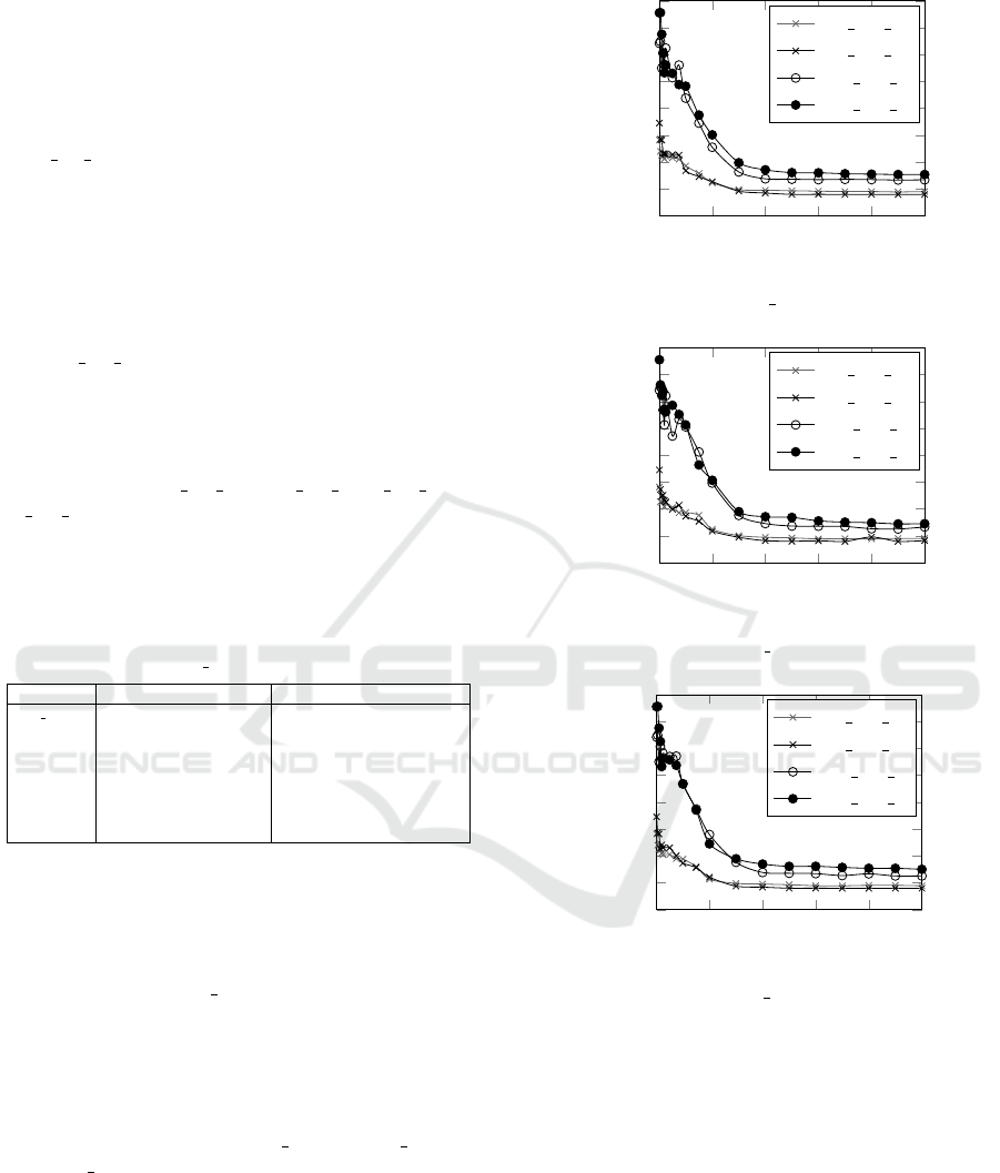
Figure 1: Improvement of average solution quality over suc-
cessive generations.
parameter values for all instances. One may study
(Birattari, 2005; Eiben and Smith, 2011) for a de-
tailed coverage of parameter tuning in metaheuristic
techniques in general. It should be noted that all val-
ues of parameters are same for each variant of ACO
approach, as it was observed experimentally that each
variant of ACO approach produces high quality solu-
tion overall.

Table 2: Results of three variants of ACO approach on different graph instances for the [Tree] t-SP.
Instance Characteristics ACO Local ACO Global ACO Mixed
Vertex Edge Best Avg SD ATET Best Avg SD ATET Best Avg SD ATET
50 0.0 1 50 0% 4.92 4.97 0.04 6.53 4.73 5.19 0.29 6.74 4.92 4.97 0.05 6.54
50 0.2 1 50 20% 4.49 4.58 0.08 8.15 4.51 4.63 0.10 8.40 4.44 4.56 0.06 8.16
50 0.4 1 50 40% 4.53 4.57 0.04 6.66 4.53 4.77 0.25 6.88 4.44 4.54 0.06 6.66
50 0.6 1 50 60% 4.64 4.83 0.21 4.65 4.74 5.08 0.21 4.81 4.57 4.71 0.13 4.66
50 0.0 2 50 0% 5.02 5.19 0.17 6.52 5.11 5.32 0.20 6.75 5.02 5.27 0.13 6.53
50 0.2 2 50 20% 4.69 4.79 0.11 7.93 4.70 4.96 0.20 8.24 4.69 4.82 0.16 7.93
50 0.4 2 50 40% 3.98 4.04 0‘06 6.61 4.13 4.47 0.24 6.85 3.98 4.19 0.23 6.62
50 0.6 2 50 60% 4.05 4.07 0.03 4.57 4.04 4.42 0.27 4.73 4.05 4.06 0.02 4.59
50 0.0 3 50 0% 5.45 5.63 0.09 6.61 5.45 5.91 0.39 6.77 5.45 5.69 0.13 6.56
50 0.2 3 50 20% 4.87 4.91 0.02 8.22 4.85 5.01 0.15 8.47 4.87 4.91 0.02 8.22
50 0.4 3 50 40% 4.87 4.91 0.02 8.22 4.85 5.01 0.15 8.49 4.87 4.91 0.02 8.22
50 0.6 3 50 60% 4.38 4.52 0.08 4.64 4.43 4.70 0.23 4.79 4.26 4.50 0.14 4.64
100 0.0 1 100 0% 6.54 6.91 0.22 45.37 6.71 7.04 0.24 45.55 6.67 6.83 0.17 45.28
100 0.2 1 100 20% 6.71 6.83 0.08 62.40 6.66 6.92 0.24 64.66 6.28 6.66 0.18 62.36
100 0.4 1 100 40% 6.49 6.83 0.22 51.20 6.24 6.92 0.46 52.81 6.42 6.68 0.18 51.00
100 0.6 1 100 60% 6.80 7.40 0.33 34.51 6.64 7.09 0.29 35.65 6.77 7.22 0.37 34.55
100 0.0 2 100 0% 6.66 6.76 0.08 45.50 6.66 6.99 0.29 45.47 6.39 6.55 0.13 45.48
100 0.2 2 100 20% 6.23 6.47 0.19 62.83 6.04 6.80 0.40 62.76 6.18 6.39 0.11 62.82
100 0.4 2 100 40% 6.06 6.19 0.16 50.84 6.10 6.61 0.49 50.92 6.09 6.20 0.15 50.95
100 0.6 2 100 60% 5.97 6.12 0.16 34.51 6.21 6.65 0.33 35.74 5.98 6.19 0.18 34.51
100 0.0 3 100 0% 8.07 8.73 0.15 45.69 7.51 8.12 0.41 45.52 7.60 8.08 0.21 45.59
100 0.2 3 100 20% 7.71 7.93 0.20 63.16 7.49 8.83 0.61 63.30 7.58 7.89 0.17 63.14
100 0.4 3 100 40% 7.70 7.89 0.18 51.19 7.27 7.90 0.46 52.98 7.51 7.78 0.17 51.04
100 0.6 3 100 60% 7.53 7.93 0.17 34.38 7.25 7.53 0.28 35.67 7.38 7.73 0.23 34.39
4.3 Performance Evaluation
Table 2 reports the results of each variant of
ACO approach (i.e., ACO Local, ACO Global, and
ACO Mixed) for the [Tree] t-SP on a set of graph
instances. In Table 2, column Instance denotes the
name of each graph instance in A1 A2 A3 format;
columns Vertex and Edge respectively denote the to-
tal number of vertices and edges of the graph; and
columns Best, Avg and SD and ATET, respectively de-
note the best value, the average value, the standard
deviation and the average total execution obtained by
ACO Local, ACO Global, and ACO Mixed over 10
runs.
One can also observe in Table 2 that among all
three variants of ACO approach, ACO Local, in terms
of Best, is better on 3, is equal on 4 and is worse on
17 graph instances in comparison to other variants of
ACO approach; ACO Local, in terms of Avg, is better
on 6, is equal on 3 and is worse on 15 graph instances
in comparison to other variants of ACO approach;
ACO Global, in terms of Best, is better on 11, is equal
on 1 and is worse on 12 graph instances in compari-
son to other variants of ACO approach; ACO Global,
in terms of Avg, is better on 2 and is worse on 22 graph
instances in comparison to other variants of ACO ap-
proach; ACO
Mixed, in terms of Best, is better on 6,
is equal on 4 and is worse on 14 graph instances in
comparison to other variants of ACO approach; and
ACO Mixed, in terms of Avg, is better on 13, is equal
on 3 and is worse on 8 graph instances in comparison
to other variants of ACO approach. Based on experi-
mental observation, ACO Global is better in terms of
Best and in terms of Avg ACO Mixed is better; how-
ever one can also notice that the results obtained by
all three variant of ACO approaches are close to each
other.
4.4 Convergence Analysis
To examine the effectiveness of the proposed three
variants of ACO approach for the [Tree] t-SP, we have
performed experiments based on convergence of each
proposed variant of ACO approach. For this, four
graph instances i.e. 50 0.4 1, 50 0.4 2, 100 0.2 1 and
100 0.4 3 have been selected from the set of consid-
ered graph instances. Figure 1-(a-c) respectively de-
pict the emergence of average solution quality (av-
erage value (Avg) based on 10 runs) over succes-
sive generations. The curves in Figure 1-(a-c) clearly
demonstrate that the proposed three variants of ACO
approach for this problem converge rapidly towards
the high quality solution.
5 CONCLUSIONS
This paper concerns the tree t-spanner problem for
connected, undirected and weighted graph and pro-

poses three variants of ACO approach. All compo-
nents of each variant of ACO approach are the same
except the updating rule regarding the pheromone
trails component. All three variants of ACO ap-
proach have been tested on a set of randomly gen-
erated graph instances. Experimental results demon-
strate the effectiveness of solution quality obtained by
all three variants of ACO approach on each instance.
It was also found empirically that the performance
of all three variants of ACO approach are close to
each other. Convergence analysis on some instances
show that all three variants of ACO approach con-
verge rapidly towards the high quality solutions over
successive generations for such instances.
As a future work, other metaheuristic techniques
will be developed for this problem, as this problem
is under-studied in the domain of metaheuristic tech-
niques.
ACKNOWLEDGEMENTS
This work is supported in part by a grant (grant num-
ber YSS/2015/000276) from the Science and Engi-
neering Research Board – Department of Science &
Technology, Government of India.
REFERENCES
Alth
´
ofer, I., Das, G., Dobkin, D., Joseph, D., and Soares, J.
(1993). On sparse spanners of weighted graphs. Dis-
crete Comput. Geom., 9:81–100.
Awerbuch, B., Baratz, A., and Peleg, D. (1992). Efficient
broadcast and light-weight spanners.
Bhatt, S., Chung, F., Leighton, F., and Rosenberg, A.
(1986). Optimal simulations of tree machines. In Pro-
ceedings of 27th IEEE Foundation of Computer Sci-
ence, pages 274–282.
Birattari, M. (2005). Tuning Metaheuristics: A Machine
Learning Perspective. Springer-Verlag.
Cai, L. (1992). Tree spanners: Spanning trees that approxi-
mate distances.
Cai, L. and Corneil, D. (1995). Tree spanners. SIAM J.
Discrete Math., 8:359–387.
Dorigo, M., Maniezzo, V., and Colorni, A. (1991). Positive
feedback as a search strategy. Technical Report 91-
016, Dipartimento di Elettronica, Politecnico di Mi-
lano, Milan, Italy.
Dorigo, M. and St
¨
utzle, T. (2004). Ant Colony Optimiza-
tion. MIT Press, Cambridge, MA.
Dragan, F. F. and K
¨
ohler, E. (2014). An approximation al-
gorithm for the tree t-spanner problem on unweighted
graphs via generalized chordal graphs. Algorithmica,
69:884–905.
Eiben, A. E. and Smith, S. K. (2011). Parameter tun-
ing for configuring and analyzing evolutionary algo-
rithms. Swarm and Evolutionary Computation, 1:19–
31.
Emek, Y. and Peleg, D. (2008). Approximating minimum
max-stretch spanning trees on unweighted graphs.
SIAM J. Comput., 38:1761–1781.
Harel, D. and Tarjan, R. (1984). Fast algorithms for finding
nearest common ancestors. SIAM J. Comput., 13:338–
355.
Liebchen, C. and W
¨
unsch, G. (2008). The zoo of tree
spanner problems. Discrete Applied Mathematics,
156:569–587.
Liestman, A. and Shermer, T. (1993). Additive graph span-
ners. Networks, 23:343–364.
Moharam, R. and Morsy, E. (2017). Genetic algorithms to
balanced tree structures in graphs. Swarm and Evolu-
tionary Computation, 32:132–139.
Monteiro, M. S. R., Fontes, D. B. M. M., and Fontes, F.
A. C. C. (2015). The hop-constrained minimum cost
flow spanning tree problem with nonlinear costs: an
ant colony optimization approach. Optimization Let-
ters, 9:451–464.
Peleg, D. and Tendler, D. (2001). Low stretch spanning
trees for planar graphs.
Peleg, D. and Ullman, J. (1987). An optimal synchronizer
for the hypercube. In Proceedings of 6th ACM Sym-
posium on Principles of Distributed Computing, Van-
couver, pages 77–85.
Peleg, D. and Upfal, E. (1988). A tradeoff between space
and efficiency for routing tables. In Proceedings
of 20th ACM Symposium on Theory of Computing,
Chicago, pages 43–52.
Prim, R. (1957). Shortest connection networks and some
generalizations. Bell Systems Technical Journal,
36:1389–1401.
Sundar, S. and Singh, A. (2013). New heuristic approaches
for the dominating tree problem. Applied Soft Com-
puting, 13:4695–4703.
Sundar, S., Singh, A., and Rossi, A. (2012). New heuris-
tics for two bounded-degree spanning tree problems.
Information Sciences, 195:226–240.
Venkatesan, G., Rotics, U., Madanlal, M. S., Makowsky,
J. A., and Rangan, C. P. (1997). Restrictions of min-
imum spanner problems. Information and Computa-
tion, 136:143–164.
