Impact of Hidden Weights Choice on Accuracy of MLP with
Randomly Fixed Hidden Neurons for Regression Problems
Marie-Christine Suhner
1,2
and Philippe Thomas
1,2
1
Université de Lorraine, CRAN, UMR 7039, Campus Sciences, BP 70239, 54506 Vandœuvre-lès-Nancy cedex, France
2
CNRS, CRAN, UMR7039, France
Keywords: Neural Network, Extreme Learning Machine, Multilayer Perceptron, Parameters Initialization, Randomly
Fixed Hidden Neurons.
Abstract: Neural network is a well-known tool able to learn model from data with a good accuracy. However, this tool
suffers from an important computational time which may be too expansive. One alternative is to fix the
weights and biases connecting the input to the hidden layer. This approach has been denoted recently
extreme learning machine (ELM) which is able to learn quickly a model. Multilayers perceptron and ELM
have identical structure, the main difference is that only the parameters linking hidden to output layers are
learned. The weights and biases which connect the input to the hidden layers are randomly chosen and they
don’t evolved during the learning. The impact of the choice of these random parameters on the model
accuracy is not studied in the literature. This paper draws on extensive literature concerning the feedforward
neural networks initialization problem. Different feedforward neural network initialisation algorithms are
recalled, and used for the determination of ELM parameters connecting input to hidden layers. These
algorithms are tested and compared on several regression benchmark problems.
1 INTRODUCTION
Since the backpropagation algorithm proposed by
Rumelhart and McClelland (1986), neural networks
have shown their abilities to solve a broad array of
problem including regression, classification,
clustering as examples. However, the design of a
neural model needs a learning step which may be
very computational time consuming. To overfit this
drawback, Schmidt et al., (1992) have been the firsts
to proposed to adapt only the weigths and biases
connecting the hidden to the output layers. Huang et
al., (2004) have formalised this approach and called
it: Extreme Learning Machine (ELM). This tool has
been the subject from many publications, including
theoretical purpose (Lendasse et al., 2016) or
application (Rajesh and Parkash, 2011).
ELM structure is similar to structure of classical
single hidden layer feedforward neural network.
Multilayer perceptron (MLP) uses backpropagation
algorithm in order to adapt all the parameters
(weights and biases connecting the input to the
hidden layers and those connecting the hidden to the
output layers). Rather, in ELM, the weights and
biases connecting the input to the hidden layers are
fixed and only those connecting the hidden to the
output layers constitute the parameters set which are
tuned by using one-pass algorithm. This fact leads to
a great improvement of the learning computational
time. Even if some authors claim that ELM
preserves their habilites of universal aproximator
(Huang and Lai, 2012; Javed et al., 2014), Li and
Wang (2017) have proved that it was not true.
However, ELM preserves their interest due to their
good capabilities to deal with large data analysis,
fast dynamic modelling and real–time data
processing (Cui and Wang, 2016).
The choice of the hidden nodes impacts the ELM
accuracy (Huang and Lai, 2012, Feng et al., 2009,
Qu et al., 2016). To improve it, many researchers
focus on the hidden nodes number determination by
using genetic algorithm (Suresh et al., 2010),
pruning procedure (Miche et al., 2010) or
incremental learning approaches (Feng et al., 2009).
The random choice of the weights and biases
connecting the input to the hidden layers is rarely
discussed. We can cite Qu et al., (2016) which
distinguish classification problems where orthogonal
initialisation allows to improve accuracy, when
better results are obtained if random initialisation is
Suhner M. and Thomas P.
Impact of Hidden Weights Choice on Accuracy of MLP with Randomly Fixed Hidden Neurons for Regression Problems.
DOI: 10.5220/0006495702230230
In Proceedings of the 9th International Joint Conference on Computational Intelligence (IJCCI 2017), pages 223-230
ISBN: 978-989-758-274-5
Copyright
c
 2017 by SCITEPRESS – Science and Technology Publications, Lda. All rights reserved

used for regression problems. The great majority of
works related to ELM include a simple random
initialisation of these weights and biases (Huang et
al., 2004; Huang et al., 2006). Some works proposed
a more sophiticated initialisation procedure (Javed et
al., 2014) including the use of evolutionary
algorithms (Evolutionary-ELM) which may
deteriorate the computational time (Zhu et al., 2005,
Cao et al., 2012; Matias et al., 2014). At the oposite,
other works do not say a word about this problem
(Huang and Lai, 2012; Yin et al., 2015).
On the contrary, in the MLP context, the problem
of initialization of the weigths and biases connecting
the input to the hidden layers have been studied
(Nguyen and Widrow, 1990; Burel, 1991; Drago and
Ridella, 1992; Thomas and Bloch, 1997).
In this paper, the impact of the using of
sophisticated MLP initialization algorithms for ELM
model accuracy for regresion purpose is
investigated. Next section will present the structure
and the learning algorithm of the considerd ELM.
The hidden nodes choice is also discussed. Section
three recalls five MLP initialization algoritms. These
algorithms are used for ELM models for three
regresion benchmarks in section four before to
conclude.
2 EXTREME LEARNING
MACHINE (ELM)
2.1 ELM Structure and Notations
The structure of an ELM is similar to the MLP
structure and is given by:

011
1
0
11 1
2
1
.. ..
.1...
nnn
kki ihh kii
ih i
n
ki i
i
zwgvx wVX
wH with k n
 






 

(1)
where,
k
z
are the
2
n
outputs and
0
h
x
are the n
0
inputs
of the ELM (
0
0
n
x
is a constant input equal to 1),
ih
v
are the weights connecting the input layer to the
hidden layer,
g(.) is the activation function of the
hidden neurons,
ki
w are the weights connecting the
hidden neurons to the output
k,
i
H
is the is the
output of the hidden neuron
i (
1
n
H
is a constant
input equal to 1). Equation 1 is written compactly as:
.
Z
WH
(2)
where
Z is the estimated output matrix:
1
1
(1) (1)
() ()
o
o
n
n
zz
Z
zN z N











(3)
H is the hidden layer output matrix:






1
1
1
,..., , (1),..., ( )
.(1) .(1)
.() .()
n
h
h
N
n
n
HV V X XN
gVX gV X
gVX N gV XN













(4)
and W the ELM parameters matrix:
2
1
T
T
n
W
W
W











(5)
Different activation functions have been proposed
for the hidden nodes (Javed et al. 2014). In this
paper, initialization algorithms are tested for ELM
regression models. So the classical hyperbolic
tangent is chosen.
2.2 ELM Learning Algorithm
Different learning algorithms have been proposed to
determine the parameters of the model. The one used
here is summarized as follow (Huang et al., 2006):
 The weights
ih
v and biases
1
i
b connecting the
input to the hidden layers are randomly selected.
 Calculate the hidden layer output matrix H by
(4). Calculate the ELM parameters by using
H
†
the Moore-Penrose generalized inverse of matrix
H (Huang et al., 2006):
.WHY
†
(6)
Many modification have been proposed to
improve accuracy of such learning algorithms as
robust ELM (Zhang and Luo, 2015), regularized
ELM (Deng et al., 2009), incremental (Huang et al.,
2006), regularized incremental (Xu et al., 2016).
In this paper, the goal is to test MLP
initialization algorithms. So the basic ELM
algorithm (Huang et al., 2006) is sufficient here.

H
5
H
8
H
10
H
7
-10 -8 -6 -4 -2 0 2 4 6 8 x
-1
-0.8
-0.6
-0.4
-0.2
0
0.2
0.4
0.6
0.8
1
H
1
H
9
H
4
H
2
H
3
H
6
Figure 1: Hidden neurons outputs for the “SinC” problem.
2.3 Impact of Hidden Nodes Choice
The classical “SinC” example is used to illustrate the
impact of hidden nodes choice:
sin( ) / 0
()
10
xxx
yx
x






(7)
Two datasets including 1000 pairs (x
n
, y
n
) each, are
built for the learning and the validation. The x
n
are
uniformly randomly distributed between -10 and 10
and the learning dataset is polluted by a random
noise uniformly distributed between -0.2 and 0.2.
The ELM includes 10 hidden neurons (plus one
hidden node constant and equal to 1). The
parameters of these hidden nodes are randomly
uniformly distributed between -1 and 1.
Figure 1 presents the output H
i
of the 10 hidden
nodes for the validation datasets. Five of them
require a particular attention: H
5
, H
8
and H
10
on the
one hand, and H
6
and H
7
on the other hand.
First, it appears that H
5
, H
8
and H
10
are near to be
constant on the considered input domain and are not
significantly different to the bias node H
11
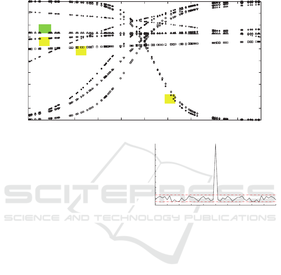
. Second,
the outputs H
6
and H
7
seems very similar. So, a cross
correlation test is performed on these two outputs
and presented figure 2. This correlation test confirms
that these two hidden neuron outputs are closely
correlated. So, only one of them gives information.
So despite the fact that we include ten hidden
nodes in the model, only six of them are really
useful. To comfirm this fact, the accuracy of two
models is compared on the validation dataset. The
first ELM model includes all the hidden nodes and
-25 -20 -15 -10 -5 0 5 10 15 20 lag
-0.1
0
0.1
0.2
0.3
0.4
0.5
0.6
0.7
0.8
0.9
Figure 2: Cross correlation between H
6
and H
7
.
the resulting sum squared errors (SSE) is equal to
1.51*10
-4
. The second ELM model includes only six
hidden nodes (H
5
, H
6
, H
8
and H
10
are discarded).
The SSE obtained for this model is 2.23*10
-4
. The
difference between the results obtained is not
statistically significant.
This experience shows that even if the
parameters are randomly choosen, a lack of diversity
may lead to the fact that some of the hidden nodes
are unuseful. To make an analogy with classifiers
ensembles, the accuracy of the ELM depends on the
diversity of its individual components (hidden
nodes) (Kuncheva and Whitaker, 2003). That’s why
ELM needs a good initialization algorithm in order
to improve diversity between the hidden nodes.
3 MLP INITIALISATION
ALGORITHMS
Many algorithms have been proposed in the past in
order to initialize MLP.

3.1 Random Initialization (Ra)
Random initialization has been the first approach to
initialize parameters since the pioneering work of
Rumelhart and McClelland (1986). This approach is
mainly used in ELM approach since the work of
Huang et al., (2004). This approach consist to
uniformly randomly initiate the parameters between
–r and r. Initially, nothing is said about the value of
r. In this paper, r is tuned to 1 in accordance with
settings encountered in the literature (Norgaard,
1995, Zhu and Huang, 2004). This algorithm will be
denoted “Ra” in the sequel.
3.2 Burel Initialization (Bu) (Burel
1991)
The arbitrarily setting of r has been discussed in the
past and researchers have exploited some
information to tune it. Within this philosophy, Burel
(1991) searches to give an equivalent influence for
each hidden neuron on the model accuracy. To do
that, the weights and biases connecting the input to
the hidden layers must be tuned such that:
1
2
1
(1) (. ()) 0 1, ,
(2) var(. ()) 1, ,
i
iz
CEVXn i n
CVXn in






(8)
Satisfy the requirement C1 allows to use the full
variation of the activation range. C2 serves to
control the variation amplitude range. C1 is
validated if the two bounds r and –r are
symmetrical. To respect C2, r must be tuned to:




0
0
2
2
2
1
1
3
0.87
z
n
n
h
h
h
h
r
Ex
Ex






(9)
z

is tuned to 0.5 because the hyperbolic tangent is
nearly linear between -0.5 and 0.5. This tuning of r
implies that this initialisation algorithm requires a
complete dataset. This initialization algorithm will
be denoted “Bu”.
3.3 Drago and Ridella Initialization
(DR) (Drago and Ridella, 1992)
Within the same philosophy as Burel (1991), Drago
and Ridella (1992) search to find a good tuning of r.
They tried to control the proportion of samples in
the dataset leading to the saturation of the activation
function. They defined the “Paralyzed Neuron
Percentage” (PNP) which represent the proportion
of samples leading to obtain paralyzed neuron(s).
They found a relation between this parameter and r:
1
3
1
.
22
r
erf PNP







(10)
where
1/

represents the probability that at least
one output of the network is incorrect:
11
1
2
o
N





(11)
The goal of this algorithm is to maintain the PNP to
a small value. So PNP is tuned to 5% in (10). This
initialisation algorithm needs a complete dataset. It
will be denoted “DR” in the sequel.
3.4 Nguyen and Widrow Initialization
(NW) (Nguyen and Widrow, 1990)
Nguyen and Widrow (1990) algorithm can be view
as a slice linearization. Its goal is to determine
parameters such that all hidden nodes represents a
linear function on a small interval of the input space.
To do that, the size of the intervals and their
localisation in the input space must be determined.
The size is controlled by the amplitude of the
weights vectors
0
11
'
iiin
Vvv






, i=1, n
1
-1 (not
including biases
0
in
v
) when the localisation is
controlled by the biases
0
in
v
of the hidden neurons.
In order to break the symmetry in the network,
all the weights and biases are randomly uniformly
distributed between -1 and 1. In a second step, the
amplitude of the weights vectors
'
i
V
are adjusted in
function of the number of inputs and hidden units:
0
1/
1
'0.7*
n
i
Vn
(12)
Multiplying by 0.7 gives a slight overlapping of the
intervals. The localisation of the intervals in the
input space is determined by the tuning of the biases
of the hidden neurons
0
in
v
. They are uniformly
randomly chosen in the range
', '
ii
VV


.
Initially, this algorithm has been designed in
order to work with normalised inputs between -1 and
1. In order to work with no normalized inputs,
Demuth and Beale (1994) have implemented an
improvement of this algorithm in matlab®. To do
that, each weight
ih
v , i=1, …, n
1
-1, and h = 1, …, n
0-
1
, are divided by the amplitude of the input h:

max( ) min( )
2
hh
h
x
x



(13)
The centres of the intervals are repositioned in the
input space by adding to the biases of the hidden
neurons
0
in
v
:
0
00
1
min( ) max( )
2
n
ihi
h
x
x
v





(14)
This algorithm requires to know the amplitude of
each input. It will be denoted “NW” in the sequel.
3.5 Chen and Nutter Initialization (CN)
(Chen and Nutter, 1991)
Chen and Nutter (1991) proposed a totally different
approach. They tried to estimate the initial
parameters of each layers sequentially. The main
problem is that the outputs of the hidden neurons are
unknown. So Chen and Nutter proposed to initialize
the parameters in different stages. First all the
parameters are randomly uniformly distributed
between -1 and 1. Second, parameters which connect
the hidden to the output layers are estimated:
1
(.)..
TT
WHHHT


(15)
Third, the desired output T is retro propagated to the
hidden neurons:








1
1
1
if rank
.
rank
if rank
.( . ) .
rank
if rank
..(.)
rank
TT
T
h
TT
TT
h
TT
TT
WT
TW
WN
WT
HTWWW
WN
WT
TW WW
W




























(16)
The estimated outputs of the hidden neurons are
finally obtained by mixing information given by
output and by inputs:
.
H
HH


(17)
with
 , a parameter chosen randomly between 0 and
1. This estimation of the hidden neurons outputs
may lead to values outside the bounds -1, 1. These
value must be truncated between -1 and 1.
Fourth, the parameters connecting the input to
the hidden layers are estimated:


















11
1
1
1
1
1
1
1
ˆ
ˆ
.
if rank
rank
ˆ
ˆ
.. .
if rank
rank
ˆ
ˆ
...
if rank
rank
T
h
h
i
TT
h
h
i
TT
h
h
V
XgH
XgH
X
N
XXX gH
XgH
X
N
XX Xg H
XgH
X































(18)
This algorithm needs a complete dataset. It will be
denoted “CN”.
4 EXPERMENTAL RESULTS
The five MLP initialisation algorithms are tested in
order to initialize ELM model on three regression
benchmarks. For each initialization algorithm and
for each benchmark, twenty initial parameters sets
are built. For each benchmark, the number of hidden
neurons is fixed according to the studies of Huang et
al., (2006).
4.1 Comparison Criterion
The selection criterion used to compare the results
obtained is the classical Root Mean Square Error
(RMSE):

2
1
1
() ()
N
n
RMSE t n z n
N



(19)
However, two values of RMSE may be sufficiently
close such that the difference is statistically
insignificant. So to compare two ELM models, their
residuals populations P
0
and P of mean 0 and of
variance
2
0

and
2

respectively must be compared
by using a two tailed hypothesis test in order to
determine if
2

is statistically different of
2
0

. The
null hypothesis
0
H
(the two variance are
statistically equal) and its alternative
1
H
are:
22
0
0
22
1
0
22
0
:
:














H
H
(20)
0
H
is rejected with a risk level of 5% if:



2
2
1
2
0
2
2
2
2
0
1.
,
2
1.
,1
2
c
c
N
N











  








   




(21)
where
 is the number of degree of freedom, and 
is the confidence level.
4.2 Abalone Dataset
This abalone dataset is a collection of 4177 samples
and the goal is to predict the age (output) of these
shells considering eight physical measurements
(inputs) (Waugh, 1995; UCI, 2017). From these
4177 samples, 2000 are used for the learning and
2177 for the validation. The output is normalised
between -1 and 1. No normalisation is performed on
the inputs. Table 1 presents the results obtained for
all the ELM models.
The first row of table 1 presents the mean
computational time for each algorithm. Four of them
presents a very short and similar computational time
(Bu, DR, NW and Ra). These four algorithms are
very simple, when CN performs least square
calculus twice.
The six succeeding rows give respectively the
min, mean and max values of RMSE on the learning
and the validation datasets. The best RMSE value on
the learning and validation datasets is given by Bu.
For the validation dataset, Ra gives the same
optimum. So, Bu and, to a lesser extent Ra, give the
best results concerning the RMSE value.
However, it is likely that some of the other
results are statistically equal to the best one. The two
bounds
1c

and
2c

of the statistical test (21) are
equal to 2050 and 2308 respectively for this
example. The last row of table 1 presents the
proportion of ELM models which gives a RMSE
statistically equivalent to the best one on the
validation data set (here best Bu model).
Only three initialisation algorithms (Bu, NW and
Ra) are able to give results statistically equivalent to
the best one. Among them, NW is the one which
maximizes this proportion (30%).
Table 1: Results for the Abalone dataset.
Bu CN DR NW Ra
0.0016 0.0055 0.0016 0.0016 0.0016
min 0.0757 0.0868 0.0791 0.0765 0.0765
mean 0.0796 0.0906 0.0863 0.0791 0.0801
max 0.0862 0.0915 0.0926 0.0844 0.0908
min 0.0723 0.0833 0.0775 0.0731 0.0723
mean 0.0769 0.0865 0.084 0.0782 0.0773
max 0.0829 0.0875 0.0951 0.0936 0.0857
15% 0% 0% 30% 15%
computational time (s)
identification RMSE
validation RMSE
%

Table 2: Results for the Auto Price dataset.
Bu CN DR NW Ra
0.0047 0.0039 0.001 0.0023 0.001
min 0.07 0.1315 0.0687 0.0773 0.1123
mean 0.0898 0.1799 0.0827 0.0976 0.1549
max 0.1228 0.1821 0.1072 0.1211 0.1821
min 0.0663 0.1178 0.071 0.0614 0.1
mean 0.083 0.1494 0.0803 0.0891 0.1499
max 0.1073 0.1508 0.0964 0.1058 0.1508
10% 0% 15% 20% 0%
computational time (s)
identification RMSE
validation RMSE
%


Table 3: Results for the CPU dataset.
Bu CN DR NW Ra
0.0008 0.0031 0.008 0.0008 0.0008
min 0.0223 0.1058 0.0494 0.0207 0.0944
mean 0.0272 0.1076 0.0701 0.0263 0.1047
max 0.0442 0.1077 0.0884 0.0413 0.1071
min 0.0494 0.1617 0.081 0.0549 0.1537
mean 0.1293 0.1643 0.1185 0.0837 0.1622
max 0.4022 0.1645 0.142 0.1468 0.1774
15% 0% 0% 20% 0%
computational time (s)
identification RMSE
validation RMSE
%

4.3 Auto Price Dataset
This dataset regroups the price of cars (output) and
fifteen of their characteristics (inputs) (Kibler et al.,
1989; UCI, 2017). The missing values are discarding
leading to a dataset comprising 159 samples
randomly divided into 80 samples for the learning
and 79 for the validation. The output is normalized
and all ELM models include five hidden neurons.
The results of all the ELM models are presented
table 2.
The mean computational time for all algorithms
are quite similar.
The best RMSE on the learning dataset is given
by DR algorithm. But, for the validation dataset, it is
NW which gives the best one.
For the statistical test (21) the two bounds
1c

and
2c
 are equal to 56.3 and 105.5 respectively.
The last row presents the proportion of model which
give results statistically equivalent to the best one
(here best NW model).
This time, the three initialisation algorithm
which gives results statistically equivalent to the best
one are (Bu, DR and NW). NW is again the one
which maximizes chances to find good model
(20%).
4.4 CPU Dataset
The Computer Hardware dataset problem is to
predict the estimated relative performance from the
original article (Kibler and Aha, 1988; UCI, 2017).
It comprises 209 samples randomly divided into
learning dataset (100 samples) and validation one
(109 samples). There are six inputs, and the output is
normalized. Each ELM model includes ten hidden
neurons.
Table 3 presents the results obtained with the
five initialisation algorithms. The computational
time for BU, DR NW and Ra are quite similar when
the one for CN is greater.
The best RMSE value is given by NW on the
learning dataset and by Bu on validation one.
Considering the statistical test (21) (
1
82
c
 and
2
140)
c

 , these two algorithms are the only ones
which are able to gives results statistically
equivalent to the best one.
5 CONCLUSIONS
This paper presents a study about the impact of
hidden nodes choice on the ELM model accuracy.
This initialisation problem has been investigated in
the MLP context in the past and five initialisation
algorithms are recalled before to be tested and
compared for the ELM initialisation on three
regression benchmarks.
The results obtained shown that two algorithms
(Bu and NW) outperform the others in terms of
chances to obtain satisfactory results. However, even
these algorithms give acceptable results in less than
30% of the cases. This fact implies that performing
the learning of ELM model needs to be done on
several different initialisation parameters sets.
Our future works will focus on how to improve
this initialization step by combining different
initialization algorithms, particularly Bu and NW.
Another question concerns the impact of inputs
selection on the ELM accuracy. In all the
benchmarks used in this study, all the inputs are
linked with the output. When it is not the case, the
impact of these spurious inputs on the ELM model
accuracy must be studied.
REFERENCES
Burel, G., 1991. Réseaux de neurones en traitement
d’images: des modèles théoriques aux applications
industrielles, Ph.D thesis of the Université de Bretagne

Occidentale.
Chen, C.L., Nutter, R.S., 1991. Improving the training
speed of three-layer feedforward neural nets by
optimal estimation of the initial weights, Proc. of the
IJCNN International Joint Conference on Neural
Networks, Seattle, USA, july 8-12, 2063-2068.
Cui, C., Wang, D., 2016. High dimensional data
regression using lasso model and neural networks with
random weights. Information Sciences, 372, 505-517.
Deng, W., Zheng, Q., Chen, L., 2009. Regularized
extreme learning machine, Proc. of IEEE Symp. on
Computational Intelligence and Data Mining
CIDM’09, 389-395
Demuth, H, Beale, P., 1994. Neural networks toolbox
user's guide. V2.0, The MathWorks, Inc
Drago, G.P., Ridella, S., 1992. Statistically controlled
activation weight initialization, IEEE Transactions on
Neural Networks, 3, 4, 627-631.
Feng, G., Huang, G.B., Lin, Q., 2009. Error minimized
extreme learning machine with growth of hidden
nodes and incremental learning, IEEE Trans. on
Neural Networks, 20, 8, 1352-1357.
Huang, G.B., Zhu, Q.Y., Siew, C.K., 2004. Extreme
learning machine: a new learning scheme of
feedforward neural networks, Proc. of the IEEE
International Joint Conference on Neural Networks, 2,
985-990.
Huang, G.B., Chen, L., Siew, C.K., 2006. Universal
approximation using incremental constructive
feedforward networks with random hidden nodes,
IEEE trans. on Neural Networks, 17, 4, 879-892.
Huang, Y.W., Lai, D.H., 2012. Hidden node optimization
for extreme learning machine, AASRI Procedia, 3,
375-380.
Javed, K., Gouriveau, R., Zerhouni, N., 2014. SW-ELM:
A summation wavelet extreme learning machine
algorithm with a priori parameter initialization,
Neurocomputing, 123, 299-307.
Kibler, D., Aha, D.W., 1988. Instance-Based Prediction of
Real-Valued Attributes, Proc. of the CSCSI (Canadian
AI) Conference
Kibler, D., Aha, D.W., Albert, M., 1989. Instance-based
prediction of real-valued attributes, Computational
Intelligence, 5, 5157
Kuncheva, L.I., Whitaker, C.J., 2003. Measures of
diversity in classifier ensembles and their relationship
with the ensemble accuracy, Machine Learning, 51,
181–207
Lendasse, A., Man, V.C., Miche, Y., Huang, G.B., 2016.
Editorial: Advances in extreme learning machines
(ELM2014), Neurocomputing, 174, 1-3.
Li, M., Wang, D., 2017. Insights into randomized
algorithms for neural networks: practical issues and
common pitfalls. Information Sciences, 382, 170-178.
Matias, T., Souza, F., Araujo, R., Antunes, C.H., 2014.
Learning of a single-hidden layer feedforward neural
network using an optimized extreme learning machine,
Neurocomputing
, 129, 428-436.
Miche, Y., Sorjamaa, A., Bas, P., 2010. OP-ELM:
Optimally pruned extreme learning machine, IEEE
Trans. On Neural Networks, 21, 1, 158-162.
Nguyen, D., Widrow, B., 1990. Improving the learning
speed of 2-layer neural networks by choosing initial
values of the adaptive weights, proc. of the IJCNN Int.
Joint Conf. on Neural Networks, 3, 21-26
Norgaard, M., 1995. Neural network based system
identification toolbox, TC. 95-E-773, Institute of
Automation, Technical University of Denmark,
http://www.iau.dtu.dk/research/control/nnsysid.html
Qu, B.Y., Lang, B.F., Liang, J.J., Quin, A.K., Crisalle,
O.D., 2016. Two hidden-layer extreme learning
machine for regression and classification,
Neurocomputing, 175, 826-834.
Rajesh, R., Parkash, J.S., 2011. Extreme learning machine
– A review and state-of-art, International Journal of
Wisdom Based Computing, 1, &, 35-49;
Rumelhart, D.E., McClelland, J.L., 1986. Parallel
Distributed processing, MIT press, Cambridge,
Massachusetts.
Schmidt, W.F., Kraaijveld, M.A., Duin, R.P.W., 1992.
Feedforward neural networks with random weights,
Proc. of 11
th
IAPR Int. Conference on Pattern
Recognition Methodology and Systems, 2, 1-4.
Suresh, S., Saraswathi, S., Sundararajan, N., 2010.
Performance enhancement of extreme learning
machine for multi-category sparse cancer
classification, Engineering Application of Artificial
Intelligence, 23, 7, 1149-1157.
Thomas, P., Bloch, G., 1997. Initialization of multilayer
feedforward neural networks for non-linear systems
identification, proc. of the 15
th
IMACS World
Congress WC’97, Berlin, august 25-29, 4, 295-300.
UCI Center for Machine Learning and Intelligent Systems
(accessed 2017), Machine Learning Repository,
https://archive.ics.uci.edu/ml/datasets.html
Waugh, S., 1995. Extending and benchmarking Cascade-
Correlation, PhD thesis, Computer Science
Department, University of Tasmania
Xu, Z., Yao, M., Wu, Z., Dai, W., 2016. Incremental
regularized extreme learning machine and it’s
enhancement, Neurocomputing, 174, 134-142
Zhang, K., Luo, M., 2015. Outlier-robust extreme learning
machine for regression problems, Neurocomputing,
151, 1519-1527
Zhu, Q.Y., Huang, G.B., 2004. Basic ELM algorithms,
http://www.ntu.edu.sg/home/egbhuang/elm_codes.htm
l.