
FPGA Implementation of the Huber-Braun Neuron Model
Marcel Beuler
1
, Alexander Krum
2
, Werner Bonath
3
and Hartmut Hillmer
1
1
Department of Electrical Engineering and Computer Science, University of Kassel,
Wilhelmsh¨oher Allee 71-73, D-34121 Kassel, Germany
2
School of Computer Science and Engineering, University of New South Wales, NSW 2052, Sydney, Australia
3
Department of Electrical Engineering and Information Technology, University of Applied Sciences, Wiesenstr. 14,
D-35390 Giessen, Germany
Keywords:
Huber-Braun, Neuronal Network, FPGA, VHDL.
Abstract:
The Hodgkin-Huxley model (HH) describes the initiation and propagation of action potentials in neurons
closed to the biological conditions, but it is not well suited for large scale simulation of neuronal networks. In
this paper, an implementation of the Huber-Braun model is presented. It is a simplified HH-type model and
able to reproduce a wide variety of spiking patterns. An FPGA is selected as a reconfigurable hardware imple-
mentation platform to simulate the network functionality of the neurons. The 32-bit floating-point format and
computation techniques (i.e. CORDIC) instead of LUTs are used to avoid loss of physiological information.
We validated our design with a C++ program and report the synthesis result based on Xilinx Virtex 6 FPGA.
1 INTRODUCTION
In physiological research computer simulations play
an important role in analyzing the neuronal informa-
tion processing in the central nervous system. Ba-
sic elements are mathematical descriptions of neurons
and synapses with different complexity. Hodgkin-
Huxley-type neuron models generate action potentials
by voltage-gated ion channels, therefore, they closely
follow the biological concept. The original approach
has four nonlinear differential equations and postu-
lates three gating variables to model the dynamics of a
sodium and potassium channel (Hodgkin and Huxley,
1952). Its solution requires a great deal of computing
power and is thus not well suited for larger neuronal
networks. That’s why several simplified models with
reduced computing effort have been developed in the
past, and their use depends on each specific problem
(Izhikevich, 2004).
For example, the Hindmarsh-Rose model has
three nonlinear differential equations and can be used
to investigate the spiking-bursting behavior of two
electrically coupled neurons (Xia and Qi-Shao, 2005).
The FitzHugh-Nagumo model approximates the HH
system by only two differential equations (FitzHugh,
1961), but it doesn’t generate bursts, which can be
important for neuronal transmission (Izhikevich et al.,
2003). One of the simplest models of a neuron’s elec-
trical properties is the Integrate-and-Fire model. It
is based on a threshold approach instead of generat-
ing action potentials and allows large network simu-
lations, but the model is unrealistic from a physiolog-
ical point of view (Gerstner et al., 2014). In this pa-
per, we have chosen the Huber-Braun neuron model
which is also a simplified HH-type model. With tonic,
bursting, and chaotic spike patterns it can reproduce
a large amount of neuronal activity. In contrast to the
Hindmarsh-Rose or FitzHugh-Nagumo model, each
parameter has a clearly defined biological correlate.
In general, analog and digital approaches can be
used to implement neuron models. The latter are more
popular as they have the advantage of higher accuracy,
lower noise sensitivity, better testability, higher flex-
ibility, etc. (Muthuramalingam et al., 2008). In this
context, an analog circuit of a Huber-Braun neuron
has problems with the first period-doubling bifurca-
tion (Hermida et al., 2012).
Target hardware for digital implementations can
be conventional CPUs, GPUs, ASICs, and FPGAs.
Conventional CPU-based execution is much slower
in comparison to specialized hardware because of its
serial nature. GPUs can exploit the parallelism of
neuronal networks better and can be a powerful alter-
native to general purpose processors. However, they
may not be able to meet real-time requirements due to
high rates of data exchange between the neurons (Du
Nguyen, 2013). ASICs provide the best performance
regarding chip area and clock frequency, but they are
expensive and their functionality cannot be changed
after chip manufacturing. Although FPGAs are not
Beuler M., Krum A., Bonath W. and Hillmer H.
FPGA Implementation of the Huber-Braun Neuron Model.
DOI: 10.5220/0006499102470254
In Proceedings of the 9th International Joint Conference on Computational Intelligence (IJCCI 2017), pages 247-254
ISBN: 978-989-758-274-5
Copyright
c
2017 by SCITEPRESS – Science and Technology Publications, Lda. All rights reserved

as powerful as ASICs, they have the great benefit of
reconfigurability during prototyping.
Several FPGA implementations of the HH neuron
model have been implemented so far (Graas et al.,
2004); (Zhang et al., 2009); (Bonabi et al., 2014). In
this paper we present an FPGA-based processor archi-
tecture for the Huber-Braun neuron model. It is pro-
grammed in VHDL and can calculate up to 1600 neu-
rons including electrical coupling in real-time on the
Xilinx ML605 development board at 200MHz clock
frequency. To validate the design, two coupled neu-
rons as well as a 20x20 network are tuned to different
synchronization states, and these results are compared
with a C++ simulation.
2 NEURON MODEL
The four-dimensional HH equations with transfer
rates can be converted in a simplified HH model with-
out the need for a power function and, finally, in a
two-dimensional system as shown in (Postnova et al.,
2012). These simplifications are acceptable, because
the exact form of an action potential is less important
than the modulation of the fire rate and impulse pat-
terns. To consider subthreshold membrane potential
oscillations which operate independently of the spike
generation, the two-dimensional system is extended
by two additional ion channels.
Within the model, spike generation is done by an
HH-type component with a fast depolarizing sodium
ion current (index d) and a fast repolarizing potas-
sium ion current (index r) with voltage- and time-
dependent conductances g
d
and g
r
. A slow depo-
larizing sodium ion current (index sd) and a slow
repolarizing potassium ion current (index sr) with
voltage- and time-dependent conductances g
sd
and
g
sr
are responsible for subthreshold oscillations. Fi-
nally, a leakage current (index l) already known from
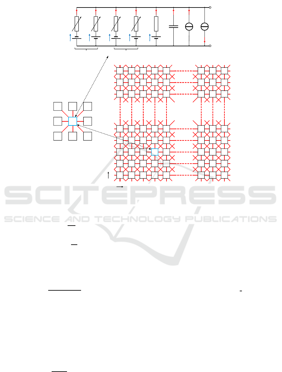
Hodgkin-Huxley is included. Figure 1 (A) shows the
equivalent circuit diagram of the neuron model with
all ion currents as well as two current sources for an
additional noise level J
noise
and the synaptic process
J
ext
. The latter one consists of a current injected ex-
ternally in the cell (J
inj
) and a gap-junction current
(J
gap
) which is explained further on.
A positive hyperpolarizing current J
ext
> 0 de-
creases the fire rate, since the membrane potential gets
more negative. With the current-voltage-relation of
the membrane capacity and Kirchhoff’s Law we get
Eq. (1). Leakage current and non-linear currents are
modeled as Eq. (4) and Eq. (5), with g
i
the conduc-
tances, a
i
the voltage- and time-dependent activation
variables, and V
i
the related Nernst potentials.
C
m
dV
dt
= −
∑
J
m
− J
ext
|
{z }
f(V)
+J
noise
(1)
∑
J
m
= J
l
+ J
d
+ J
r
+ J
sd
+ J
sr
(2)
J
ext
= J
inj
+ J
gap
(3)
J
l
= g
l
(V −V
l
) (4)
J
i
= g
i
a
i
(V −V
i
) i = {d,r,sd,sr} (5)
Similar to the HH gating mechanism, the activation
variables of the ion channels are described by differ-
ential equations first order. Steady-states are modeled
by a sigmoid curve and time constants replace the
voltage-dependent delay functions. The fast sodium
channel J
d
is instantaneous active, so a
d
= a
d∞
can be
estimated. Furthermore, J
sd
is directly coupled with
a
sr
in Eq. (9) and the related steady-state activation
a
sr∞
is omitted. Both factors ρ and ϕ are responsible
for temperature scaling of conductances g
i
and time
constants τ
i
with T
0
the reference temperature in
◦
C.
a
i∞
=
1
1+ exp[−s
i
(V −V
0i
)]
i = {d,r,sd} (6)
a
d
= a
d∞
(7)
da
i
dt
=
a
i∞
− a
i
τ
i
i = {r,sd} (8)
da
sr
dt
=
−η· J
sd
− k· a
sr
τ
sr
(9)
g
i
= g
i0
ρ = g
i0
· 1.3
(T−T
0
)/10
◦
C
(10)
1
τ
i
=
ϕ
τ
i0
=
3.0
(T−T
0
)/10
◦
C
τ
i0
(11)
Network simulations are performed by bidirectional
gap-junction coupling via J
gap
with g
gap
the coupling
strength, V
i, j
the membrane potential of an individ-
ual neuron at the position (i, j) in Figure 1 (B), and
V
i+n, j+m
the membrane potentials of neighboring neu-
rons. The summation is taken over all pairs (m,n)
with m,n ∈ {−1, 0, 1} (Postnova et al., 2009):
J
gap
i, j
=
∑
m,n
g
gap
(V
i, j
−V
i+n, j+m
) (12)
Normally, border neurons are coupled with neurons
from the opposite border to get a torus-like network:
i+ n = −1
i+ n = 40
→
→
i+ n = 39
i+ n = 0
j + m = −1
j + m = 40
→
→
j + m = 39
j + m = 0
All differential equations are solved numerically by
using the Euler integration method with ∆t = 0.1ms:
i=0
j=0
i=3
j=2
i=39
j=39
0 1
0
2 3 4 37 38 39
1
2
3
4
37
38
39
i
j
i-1
j
i
j+1
i+1
j
i+1
j+1
i+1
j-1
i-1
j+1
i-1
j-1
i
j-1
8 neighboring neurons
V
sd
V
sr
V
l
g
l
C
m
J
sr
J
sd
J
l
J
C
J
ext
V
e
V
i
g
sr
g
sd
V
d
V
r
J
r
J
d
g
r
g
d
extracellular
intracellular
spike-generation oscillations
J
noise
B
A
i=3
j=2
Figure 1: Simulated neuronal network. A) Equivalent circuit diagram of a single cell. B) Gap-junction coupling in a 40× 40
network.
V
(t+∆t)
= V
(t)
+
∆t
C
m
f(V
(t)
) + g
W
(13)
a
(t+∆t)
i
= a
(t)
i
+ ϕ
∆t
τ
i
(a
(t)
i∞
− a
(t)
i
) (14)
In Eq. (13), g
W
is a white Gaussian noise pro-
cess given by the Box-Mueller transform (Fox et al.,
1988), where a and b are two uniformly distributed
random numbers in the interval [0,1]. The noise in-
tensity can be adjusted with the parameter d.
g
W
=
p
−4d ∆tln(a) · cos(2πb) (15)
Analyzing the distribution of phase differences be-
tween spike times enables us to distinguish between
different states of synchronization in a system of es-
pecially two coupled neurons (Postnova et al., 2007).
A spike time is taken when the membrane potential
exceeds a −35mV threshold. The phase difference is
calculated by Eq. (16), wheret
1
and t
2
are the times of
subsequent spikes of the first neuron and τ is the spike
time of the second neuron (Pikovsky et al., 2001):
∆ϕ = 2π
τ−t
1
t
2
− t
1
t
1
< τ ≤ t
2
(16)
Typical values of the parameter in the above equations
can be taken from (Postnova et al., 2009).
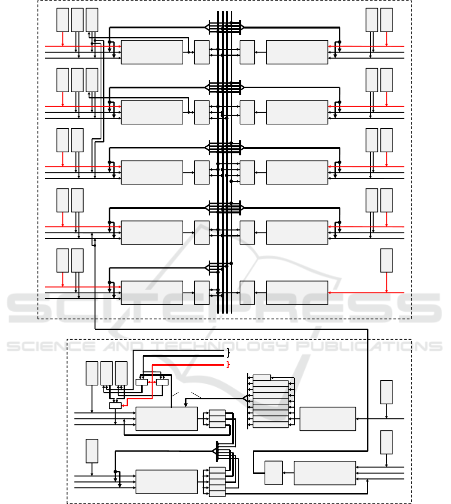
3 PROCESSOR ARCHITECTURE
Figure 2 shows the basic design of the imple-
mented architecture with two separated modules for
the Huber-Braun model equations and the electrical
synapses. It contains all necessary hardware to com-
pute 1600 neurons including gap-junction coupling
in real-time at 200MHz clock rate. Operations of
the Huber-Braun model are allocated to 9 pipelined
arithmetic units (AUs), where “ADD
SUB” is a com-
bined 12-stage adder/subtractor and “MULT” an 11-
stage multiplier. All the functions (ln, cos, sqrt, and
exp) and, in contrast to (Bonabi et al., 2014; Zhang
et al., 2009), the divisions are calculated by the it-
erative CORDIC algorithm (Walther, 1971). The re-
maining arithmetic is designed to ensure an optimum
utilization of the 50-stage CORDIC pipeline. To solve
the limited convergence domain problem of the algo-
rithm we use a unified division-free argument reduc-
tion method proposed in (Hahn et al., 1994).
Each AU processes 32-bit floating-point values
to avoid undefined effects due to significant loss of
physiological information (Zhang et al., 2009). It
has an own program memory for individually pro-

gramming of the operations, up to four FIFOs to
store the computed results and a ROM (a RAM used
as ROM after initialization) to access model-specific
parameters like g
l
and V
0r
. Two adders/subtractors
also have a RAM for the temporary storage of model
variables. These variables are the membrane poten-
tial V
(t)
(RAM of ADD
SUB A) and three activa-
tion values a
(t)
i
(RAM of ADD
SUB B), see Fig-
ure 2. OPA and OPB represent both operands for
each AU selectable by the machine instructions. To
ensure an efficient programming, the RAM content
of ADD
SUB A is provided simultaneously to a sec-
ond ADD
SUB module. FIFOs can store calculated
results in cases where a subsequent operation on the
same or another AU cannot be started immediately.
First of all, each stored FIFO result is available as an
operand for the own AU as well as all the others. Af-
ter the arithmetic operations are allocated to the indi-
vidual AUs, this wiring complexity is reduced to the
required connections in order to meet the timing spec-
ification. “PRNG” generates pseudo random numbers
via linear feedback shift registers. Here, a program
memory determines how many random numbers are
generated per time interval.
At 200 MHz clock rate, the step size of 0.1 ms is
divided into 20 identical subneuron cycles with 1000
clocks in each case. Furthermore, all subneuron cy-
cles are divided into 2 blocks with 500 clocks as the
basic execution time, i.e. all program memories with
a size of 2
9
= 512 cells can store up to 500 executable
instructions. In such a block the operations of 40
neurons are allocated to the existing hardware com-
ponents. During a neuron cycle each program mem-
ory is run through forty times with actualized index-
registers to access variables, so that 40· 2· 20 = 1600
neurons per core are computable in real-time.
Before a simulation can start, a host software has
to generate the machine instructions for each AU as
well as the ROM contents and initial states for all vari-
ables by means of the user settings. This enables us
to test different neuron models without changing the
FPGA configuration. All generated data will then be
transferred to the processor during the initialization
sequence.
Electrical Synapses. A neuron at the position (i, j)
receives 8 partial gap-junction currents from neigh-
boring neurons with J
gap
i, j
the total current. In con-
trast to Eq. (12), not each potential difference is
weighted by the coupling strength g
gap
, but only
its summation. During a block calculation of 40
neurons all synaptic operations are allocated to two
ADD
SUB modules and a multiplier. Because of
direct further processing, both ADD
SUB modules
store their results in registers. The synaptic process is
independent of the neuron model and doesn’t change,
so the related program memories have a fixed content
and cannot be modified after the FPGA is configured.
Membrane potentials are stored in two RAMs hav-
ing the same content as the ADD
SUB A-RAM of
the model equations when the initialization sequence
has finished. In each new neuron cycle, both RAMs
operate alternately by a toggle-bit, that means while
one RAM provides the membrane potentials for the
gap-junctions, the other stores the updated potentials
of the current neuron cycle parallel to ADD
SUB A-
RAM of the model equations and vice versa.
The module SET
ADDR determines the RAM
addresses of the actual neuron (Addr0) as well as
all neighboring neurons (Addr1 to Addr8) which are
identical to the neuron identification numbers (NIDs,
0···1599). These addresses are then used in the
ADD
SUB A module to select the membrane poten-
tials V
i, j
and V
i+n, j+m
with m,n ∈ {−1,0, 1}. V
i, j
is
stored in the register RegV as operand A during a
separate load instruction and the other potentials rep-
resent operand B, see Figure 2. Due to the additional
load instruction, both RAMs can be implemented as
single-port memories. The size of the neuronal net-
work can easily be adjusted by the user settings from
1× 1 to 40× 40. Eight flags define whether the po-
sitions of the neighboring neurons are located inside
the network borders and they’ve to be taken into ac-
count or not. All gap-junction currents are stored in
FIFO FGAP. Finally, these values can be accessed as
operands by the ADD
SUB D module of the model
equations.
Main-Controller. The processor has a main-
controller as higher level control which analyzes in-
coming initialization data from the host and relays
them to the related memories and registers. The
packet-based data transfer with the host is realized
by a USB 3.0 connection. A FIFO-Management-Unit
(FMU) with own buffers in both communication di-
rections controls all packet transfers between main-
controller and peripheral USB controller. Processor-
generated packets always have a length of 512 bytes
and are called PPackets to distinguish them from USB
packets (UPackets) which can have a length of 512
or 1024 bytes depending on a high-speed and super-
speed connection, respectively.
Because the processor is a 32-bit system, a 4-byte
word is processed per clock cycle. A PPacket al-
ways consists of 4 header and 124 data words. The
header contains information such as “Packet Type”
and “Packet Number”. For example, the field “Packet
Type” indicates if a certain program memory has to
be initialized or the simulation has finished. User set-
tings for core registers are summarized in a SETUP
ROM
RAM
F1A
F1B
CODE
OPA
OPB
ROM
RAM
F2A
F2B
F2C
CODE
OPA
OPB
ROM
F3A
F3B
CODE
OPA
OPB
ROM
F4A
F4B
CODE
OPA
OPB
ROM
F9A
F9B
CODE
OPA
OPB
F5A
F5B
ROM
CODE
OPA
OPB
F6A
F6B
ROM
CODE
OPA
OPB
F7A
F7B
F7C
F7D
ROM
CODE
OPA
OPB
F8A
F8B
ROM
CODE
OPA
OPB
F10
CODE
A B C D
CODE
CODE
CODE
ADD_SUB_A
ADD_SUB_B
ADD_SUB_C
CODE
ADD_SUB_D
CODE
CORDIC
CODECODECODECODECODE
PRNG
MULT_D
MULT_C
MULT_B
MULT_A
RegA
CODE
OPA
OPB
CODE
OPA
OPB
CODE
FGAP
CODE
OPA (ggap)
OPB
CODE CODE
ADD_SUB_A
ADD_SUB_B
CODE
CODE
MULT_A
SET_ADDR
RegB
RAM
RAM
RegE
RegD
RegC
RegF
RegG
updated membrane potential
Addr2/Flag2
Addr3/Flag3
Addr4/Flag4
Addr5/Flag5
Addr6/Flag6
Addr1/Flag1
Addr0
Addr7/Flag7
Addr8/Flag8
related RAM address
RegV
ADD_SUB_A (ModelEquations)
addresses of
neighbour neurons
and current neuron
MUX MUX
MUX
toggle
Core-Controller
Electrical Synapses
Model Equations
Figure 2: Block diagram of the main arithmetic components with two modules for the actual equations and the electrical
synapses. In contrast to the synapses, all program memories for the Huber-Braun equations are programmable by means of
user settings. A main-controller as higher level control and the core-controller to generate data packets for the host are not
shown.
packet. It mainly includes the mode, the selected neu-
ron model, the gap-junction networking (torus / no
torus), the network size, the threshold for spike de-
tection, as well as initial values for the ramp func-
tion g
gap
, T, and J
inj
. During run-time, each ramp
function enables an automatic incrementation of its
parameter until maximum is reached. The param-
eter interval is divided into 1000 steps, this means
∆P = (P
max
− P
init
)/1000 with P ∈ {g
gap
,T,J
inj
} and
P
max
≥ P
init
. All ramp functions determine important
tuning parameters for network analysis.
Core-Controller. During run-time, the core-

Buffer
FlagRd
Buffer
Control
Main
Controller
Rd
FMU
Control Unit
FIFO_OUT
FlagWr
TrigWr
WrAck
Rd
Data
USB
Device
Core
Controller
Model
Equations
Electrical
Synapses
ctrl
V
V
J
gap
FIFO_OUT
Neuron Core
Figure 3: Block diagram of the processor architecture. All
arithmetic components and the core-controller are summa-
rized to a neuron core.
controller increments the program counters of all
AUs, updates the ramp functions, alternates the RAM
access for gap-junctions via a toggle-bit, and com-
poses all PPackets to be transferred to the host in a
small buffer which can be read by the main-controller,
see Figure 3. Here, both modules for the actual equa-
tions and the electrical synapses as well as the core-
controller are summarized to a neuron core. Such a
core includes all necessary hardware for 1600 neu-
rons and supports several modes defining how the
calculated results are further processed in the core-
controller. In this paper, we mostly use an event-
driven mode called Preselected-Neuron-Spike-Time
(PNST). It contains the spike time and the related
NIDs of up to 124 individually selectable neurons.
With these spike times the host software can deter-
mine interspike intervals (ISI) and phase differences
according to Eq. (16), since the necessary comput-
ing power is limited. The mode Preselected-Network-
Integer (PNI) includes, among other things, the mean
membrane potential of all interconnected neurons
(mean field potential, MFP) as an indicator for syn-
chronization. Finally, the fire state of all neurons
at any time is composed in the mode Full-Network-
Spike-Time (FNST). This mode is used to plot the
dotted spike times of the entire network.
4 RESULTS
The presented architecture is written in VHDL and
synthesized on the Xilinx ML605 development board.
Buffer registers of memory outputs can be absorbed
by the related RAM during the synthesis process
with high logic delay of approximately 2ns. In
cases where the timing failed, this absorbtion can
be avoided by the keep attribute in the VHDL code.
Together with a minimum reset path we are able to
meet the timing constraints with a minimum period of
4.996ns. The synthesis results in Tab. 1 show that the
processor with one implemented neuron core takes
16 % of all LUT resources including the FMU. There-
fore, the used FPGA has enough resources for further
development like chemical synapses and multi-core
operation.
Due to the block-wise calculation of always 40
neurons, a neuron core is optimized for network sizes
of 40x40 in real-time and 20x20 in quadruple speed.
However, the simulation of two coupled neurons is
not efficient and should be done software-based, since
the results of the remaining neurons are rejected and
the high parallelism is left unexploited. For such cases
we have expanded our hardware to include a speedup
option which only works in PNST mode and defines
the number of calculated blocks per neuron cycle.
This is still worse than a software-based solution, but
it helps us in the evaluation period to reduce the real
simulation time for interspike intervals(ISI) from sev-
eral hours to less than 10 minutes.
To validate our design, the FPGA results are com-
pared with a C++ simulation. Figure 4 summarizes
the results of two electrically coupled neurons as well
as a 20x20 network at T = 6
◦
C. All simulations use
the coupling strength as tuning parameter from 0 to
its maximum value. The two neuron system is well
suited to study transitions between asynchronous and
different types of synchronous states. Figure 4 (A)
and (B) illustrate the interspike interval and the corre-
sponding phase difference with J
inj
= 0.045µA/cm
2
and g
gap,max
= 0.03mS/cm
2
for the FPGA in PNST
mode (left) and the C++ program (right). A compari-
son of these plots shows a good agreement between
both implementations. The injection current is se-
lected in a way that uncoupled neurons are closed to
the first period-doubling. This is the region where the
greatest variety of synchronous activity can be seen
for coupled neurons (Postnova et al., 2007). At first,
the neurons are in an out-of-phase synchronization
state with a constant phase difference (∆ϕ 6= 0,2π)
Table 1: Device utilization summary.
Slice Logic Used Available Utilization
Slice Registers 19,676 301,440 6 %
Slice LUTs 24,253 150,720 16%
Occupied Slices 8,720 37,680 23%
RAMB36E1 58 416 13%
RAMB18E1 42 832 5%
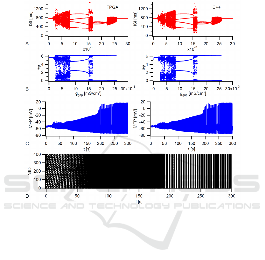
Figure 4: Simulation of two electrically coupled neurons as well as a 20×20 network at T = 6
◦
C and tuning g
gap
. A-B) FPGA
(left) and C++ (right) results for interspike intervals (ISI) and phase differences of two coupled neurons. Both simulations run
20000 s with J
inj
= 0.045µA/cm
2
and g
gap,max
= 0.03mS/cm
2
. C) FPGA (left) and C++ (right) result for the MFP of the
network with J
inj
= 0.65µA/cm
2
and g
gap,max
= 0.15mS/cm
2
. D) Dotted spike times of the FPGA network.
and a regular tonic activity. An increasing coupling
strength leads to an abruptly asynchronous behavior
with an irregular interspike interval distribution and
then to an out-of-phase state of period 4. The latter
means four lines in both diagrams. If the coupling
strength in further increased, two additional regions
with an asynchronous behavior can be seen until the
neurons go into in-phase synchronization. In general,
the simulated transitions are identical to (Postnova
et al., 2007), where more information on physiolog-
ical details can be found.
Figure 4 (C) shows, for the FPGA in PNI mode
(left) and the C++ program (right), the mean field po-
tential of a 20× 20 network with J
inj
= 0.65µA/ cm
2
and g
gap,max
= 0.15mS/cm
2
. At this injection cur-
rent, the uncoupled neurons are in the bursting
regime. Here, an increasing coupling strength leads
to a two step-like transition from the unsynchro-
nized to the fully synchronized state with a MFP
plateau at an almost synchronized state between 0.1
and 0.125mS/cm
2
. This transition was already pub-
lished for a 10× 10 network in (Postnova et al., 2009)
and makes clear that the processor works accurately.
At the end, the dotted spike times of the FPGA net-
work taken in FNST mode with synchronized bursts
at t = 250s are illustrated in Figure 4 (D).
Finally, we have compared the real simulation
time of our processor for the 20x20 network with
an Intel Core i7 (6500U) with 3.0GHz clock rate, 2
CPU-cores, and full utilization. The CPU-based sim-
ulation takes about 2.9 times longer.
5 CONCLUSIONS
We have presented a new processor architecture for
the Huber-Braun neuron model, a simplified HH-type
model. It is optimized for network sizes of 40x40

in real-time and 20x20 in quadruple speed. Synaptic
connections are realized by bidirectional gap-junction
coupling. The synthesized design runs on the Xilinx
ML605 development board at 200MHz clock fre-
quency and takes 16 % of all LUT resources. A
comparison with C++ simulations under physiologi-
cal conditions shows that the processor works accu-
rately. Furthermore, it is about 2.9 times faster than
an Intel core i7 with 2 CPU-cores. Our hierarchical
structure with a main-controller as higher level con-
trol and a neuron core with all arithmetic components
including a core-controller allows the implementation
of physiologically more relevant chemical synapses
in a special module and can easily be extended to a
multi-core architecture. This will drastically increase
the computing power and is one of the next targets of
this research.
REFERENCES
Bonabi, S., Asgharian, H., Safari, S., and Ahmadabadi, M.
(2014). FPGA implementation of a biological neural
network based on the Hodgkin-Huxley neuron model.
Frontiers in Neuroscience, 8.
Du Nguyen, H. (2013). GPU-based simulation of brain neu-
ron models. Master’s thesis, Delft Technical Univer-
sity.
FitzHugh, R. (1961). Impulses and physiological states in
theoretical models of nerve membrane. Biophysical
Journal, 1:445–466.
Fox, R., Gatland, I., Roy, R., and Vemuri, G. (1988). Fast,
accurate algorithm for numerical simulation of expo-
nentially correlated colored noise. Physical Review A,
38(11):5938–5940.
Gerstner, W., Kistler, W., Naud, R., and Paninski, L. (2014).
Neuronal dynamics - from single neurons to networks
and models of cognition. Cambridge University Press.
Graas, E., Brown, E., and Lee, R. (2004). An FPGA-based
approach to high-speed simulation of conductance-
based neuron models. Neuroinformatics, 2:417–435.
Hahn, H., Timmermann, D., Hosticka, B., and Rix, B.
(1994). A unified and division-free CORDIC argu-
ment reduction method with unlimited convergence
domain including inverse hyperbolic functions. IEEE
Transactions on Computers, 43:1339–1344.
Hermida, R., Patrone, M., Piju´an, M., Monz´on, P., Oreg-
gioni, J., and Braun, H. (2012). An analog circuit
implementation of a Huber-Braun cold receptor neu-
ron model. Conference of the IEEE Engineering in
Medicine and Biology Society, pages 3376–3379.
Hodgkin, A. and Huxley, A. (1952). A quantitative descrip-
tion of membrane current and its application to con-
ductance and excitation in nerve. Journal of Physiol-
ogy, 117:500–544.
Izhikevich, E. (2004). Which model to use for cortical spik-
ing neurons. IEEE Transactions of Neural Networks,
15(5):1063–1070.
Izhikevich, E., Desai, N., Walcott, E., and Hoppensteadt, F.
(2003). Bursts as a unit of neural information: selec-
tive communication via resonance. Trends in Neuro-
sciences, 26(3):161–167.
Muthuramalingam, A., Himavathi, S., and Srinivasan, E.
(2008). Neural network implementation using FPGA:
issues and application. International Journal of Elec-
trical, Computer, Energetic, Elecronic and Communi-
cation Engineering, 2(12):2802–2808.
Pikovsky, A., Rosenblum, M., and Kurths, J. (2001). Syn-
chronization - a universal concept in nonlinear sci-
ences. Cambridge University Press.
Postnova, S., Finke, C., Huber, M., Voigt, K., and Braun,
H. (2012). Conductance-based models for the eval-
uation of brain functions, disorders, and drug ef-
fects. InMosekilde, E., Sosnovtseva, O., and Rostami-
Hodjegan, A., editors, Biosimulation in biomedical re-
search, health care and drug development, chapter 5,
pages 97–132. Springer-Verlag.
Postnova, S., Finke, C., Jin, W., Schneider, H., and Braun,
H. (2009). A computational study of the interde-
pendencies between neuronal impulse pattern, noise
effects and synchronization. Journal of Physiology,
104:176–189.
Postnova, S., Voigt, K., and Braun, H. (2007). Neural syn-
chronization at tonic-to-bursting transitions. Journal
of Biological Physics, 33:129–143.
Walther, J. (1971). A unified algorithm for elementary func-
tions. Proc. Spring Joint Computer Conference, pages
379–385.
Xia, S. and Qi-Shao, L. (2005). Firing patterns and com-
plete synchronization of coupled Hindmarsh-Rose
neurons. Chinese Physics, 14(1):77–85.
Zhang, Y., Nunez-Yanez, J., McGeehan, J., Regan, E.,
and Kelly, S. (2009). A biophysically accurate
floating point somatic neuroprocessor. Proceed-
ings of the 2009 International Conference on Field-
Programmable Logic and Applications (FPL), pages
26–31.
