Running Race Times Prediction and Runner Performances Comparison

using a Matrix Factorization Approach

Dimitri de Smet

, Michel Verleysen

and Marc Francaux

ICTEAM, Universit

e catholique de Louvain, Louvain-la-Neuve, Belgium

IoNS, Universit

e catholique de Louvain, Louvain-la-Neuve, Belgium

Keywords:

Race Time Prediction, Athlete Evaluation, Athlete Comparison, Running, Collaborative Filtering, Matrix

Factorization.

Abstract:

This work provides tools based on matrix factorization that can be used to predict athlete running race times

based on known race results. This is of interest for athlete preparation, for workout route planning and for race

events organization. This work differentiates from previous ones by jointly considering athletes and routes.

This work shows how race records can be used to infer knowledge on the users and the races. The same tools

can also serve to compare different athlete performances and track athlete level over time. Experiments were

conducted on race records of 648 athletes from casual to elite levels. Experiments show that the methodology

can be applied to real data and gives relevant insights.

1 INTRODUCTION

More and more athletes record their sport activities

using a smartphone or a sport watch. Their records

are stored on remote servers owned by companies

that, usually, provide health or ﬁtness statistics. The

massive amount of tracks that are recorded every day

forms a basis for learning about sport practice, loca-

tions and athletes.

This paper shows how to take beneﬁt from geo-

localized running tracks to build models that can be

used to predict running race times. For this pur-

pose, this paper presents a methodology that allows

the characterization of any route in order to be able

to predict running race times of an athlete for which

a few race records are known. This is of particular

interest for race preparation and for workout route

planning. To our knowledge, previous research on

race time prediction focus on the athletes’ features

(age, morphology, gender, . . . ), the athletes’ training

measurements (Noakes et al., 1990; Vickers and Ver-

tosick, 2016; R

ust et al., 2011) or the routes’ charac-

teristics (Riegel, 1981). The framework that is pro-

posed here allows to capture complex relationships

that account for athletes and routes at the same time.

Moreover, the methodology provides tools that enable

athlete performances comparison that can be used to

compare different athletes or to track individual pro-

gression over time.

In this work, only tracks recorded during race

events are considered because they are more likely to

reﬂect athletes’ abilities than casual activities taken at

random. The task of comparing races based on race

records is not trivial because races are not attended

by the same set of athletes. Likewise, athletes’ results

cannot be compared directly because athletes do not

always attend the same races. On the other hand, there

exist some points of comparison because certain races

have some athletes in common. Making the most of

these points of comparison is related to a research area

that is called ’collaborative ﬁltering’ which includes

the well-known problem of product recommendation

(Ekstrand et al., 2011).

Experiments were performed on a small set of

races that took place in a restricted geographic area

to favor points of comparison (athletes who share sev-

eral races). Our database contains 648 users of a sport

activities sharing platform. Users recorded 276 races

over a period of two years.

2 METHOD

The methodology is divided in two main processes

that are validated individually.

First, a collection of race results is used to infer a

few underlying variables for each athlete and for each

de Smet D., Ver leysen M. and Francaux M.

Running Race Times Prediction and Runner Performances Comparison using a Matrix Factorization Approach.

DOI: 10.5220/0006499300960101

In Proceedings of the 5th International Congress on Sport Sciences Research and Technology Support (icSPORTS 2017), pages 96-101

ISBN: 978-989-758-269-1

race using matrix factorization (as it will be explained

in section 2.1). These athlete and race variables will

be referred to as athlete vectors and race vectors. It

is assumed that they synthesize the information that

is required to predict race times. Athlete vectors a

and race vectors r

are purely abstract and have no

immediate physical counterpart.

Unlike athlete vectors, race vectors are related to

objective physical quantities that are, for instance,

linked to the topology of the race. The second pro-

cess establishes a relationship between the elements

of race vectors and the actual race route character-

istics x

, like total distance or cumulative elevation

gain. Therefore, a regression model F(.) is built such

that F(x

) models as accurately as possible the r

vec-

tor produced by the ﬁrst process.

The combination of the two processes allows race

time prediction on routes that were not yet run and for

which only the itinerary is known. Indeed, route char-

acteristics x

can be computed from the itinerary; race

vectors can be obtained using the regression model

≈ F(x

) and race time for athlete a running race r

can be predicted from athlete vector a

and race vec-

tor r

2.1 Matrix Factorization

A matrix of race times (t

a,r

) with columns corre-

sponding to races and rows corresponding to athletes

is ﬁlled with known race times. In practice, most

matrix entries are unknown (over 90%) because most

athletes ran only few of the existing races. The ma-

trix factorization will allow to make predictions for

the missing values.

Race times t

a,r

are normalized with respect to race

distances d

to give the race average paces

a,r

which have better statistical distribution properties

and intuitively correspond to the notion of race difﬁ-

culty: the faster they are run, the easier they are. The

normalization also gives the advantage that the error

criterion detailed below will not favor long races.

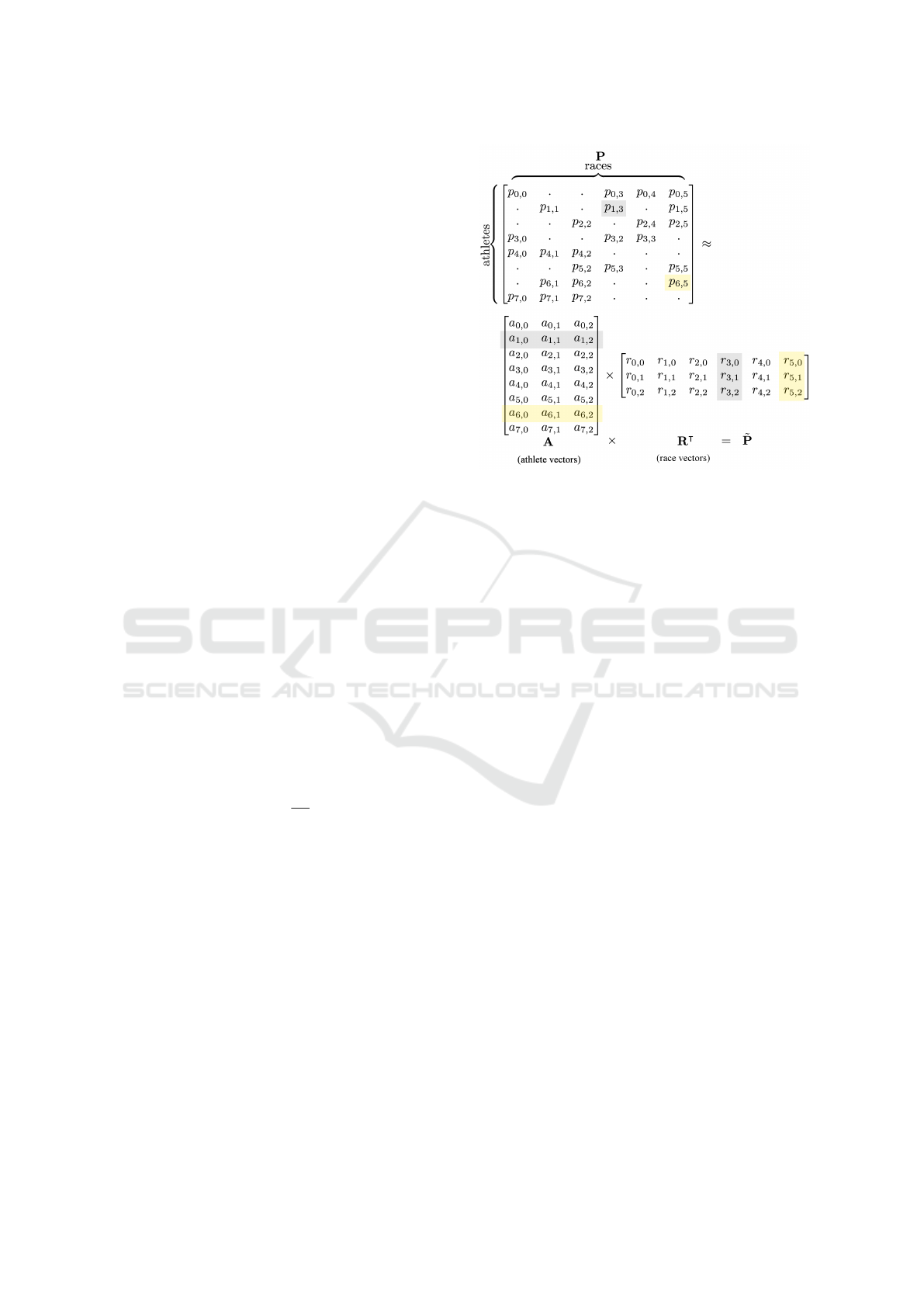
The matrix factorization depicted in Figure 1 re-

sults in an abstract vector representation of chosen

length N for each race r and for each athlete a, respec-

tively r

and a

. The vectors summarize and smooth

the information contained in the known race results.

It is postulated that the vectors can then serve to gen-

erate predictions for the missing race results.

2.1.1 Model

As shown in Figure 1, it is assumed that the average

race paces depend linearly on both race vectors r

and

Figure 1: The matrix factorization produces a vector of

length N (here N = 3) for each race and for each athlete.

Dots represent unknown entries for which predictions can

be achieved by dot product.

athlete vectors a

. Average paces p

a,r

can therefore be

expressed as a sum of N product terms

a,r

N−1

∑

i=0

a,i

· r

r,i

+ ε

a,r

(1)

where ε refers to an added noise that reﬂects the fact

that our relationship is not deterministic and only

holds true on average. Predictions can be expressed

˜p

a,r

N−1

∑

i=0

a,i

· r

r,i

. (2)

2.1.2 Optimization

The problem to be solved is to choose athletes and

races vectors that best reproduce observed average

race paces. Let Ω be the set of observed entries (a, r)

of the matrix p

a,r

. Using the least square error crite-

rion, athlete and race vectors can be found by solving

the optimization problem

min

A,R

∑

(a,r)∈Ω

a,r

− a

· r

)

. (3)

This is a non-convex problem that can be solved

using heuristics that proved to converge well in prac-

tice. Successful experiments are conducted using

stochastic gradient descent and alternate least square

algorithms. Stochastic gradient descent loops over

Ω slightly modifying A and R in the direction of the

steepest gradient; reducing the error criterion at each

step (Gemulla et al., 2011). Alternate least square al-

ternates between two convex problem: optimization

of the R vectors while holding A vectors constant

and optimization of the A vectors while holding the

R vectors constant (Jain et al., 2013) .

2.1.3 Matrix Requirements and Choice of N

Obviously, the matrix factorization cannot produce

sound vectors if the number of elements to estimate

is larger than the number of known entries. This con-

dition is met only if each race has at least N athlete

results to estimate their N vector elements and if each

athlete has at least N race results. Races and athletes

that do not fulﬁll this condition are removed from the

database. In practice, as race times account for vari-

ables that do not come into picture here (such as ath-

lete’s ﬁtness of the day or weather conditions), N vec-

tor elements require slightly more than N race results

so that the noise on the data can be averaged out.

Parameter N is related to the complexity of the

model. A small N value corresponds to a simple

model that is more likely to generalize well but that

might not capture the entire information included in

the race results matrix. A larger value of N requires

more data.

Choosing N = 1 would mean that the model as-

sumes that a race time only depends on one parameter

per race (that can be interpreted its difﬁculty) and one

parameter per athlete (that can be interpreted as the

inverse of his ﬁtness level).

Choosing N > 1 allows a multivariate representa-

tion of what makes races faster or slower and a mul-

tivariate representation of corresponding athlete abili-

ties. For instance, if vector elements can be mapped to

route characteristics, the model could express the race

difﬁculty and athlete abilities in terms of endurance,

ascent or ground surface type.

2.1.4 Matrix Factorization Validation

To quantify the ability to determine the A and R vec-

tors that approximate the known race results, 10 per-

cent of the known matrix entries are removed from the

initial set (prior to matrix factorization) and then com-

pared to the same entries in the approximated paces

matrix

P = A · R

. The process is repeated 10 times,

keeping 10 other percent apart. The accuracy is then

taken as the average root mean square error over the

10 repetitions. This process corresponds to a 10-fold

cross validation scheme (James et al., 2013).

2.2 Mapping Race Vector Elements to

Objective Route Features

The aforementioned matrix factorization gives vec-

tors of N athlete variables and vectors of N race vari-

ables. As it would be of practical use to estimate route

vectors on new routes for which race results are not

(yet) known, the known route parameters r

need to

be linked with objective route features.

2.2.1 Route Features

Routes are described as a list of geo-localized coor-

dinates to which corresponding altitudes can be asso-

ciated. Although one can argue that other parameters

can be related to race times (such as weather condi-

tions and ground type), our characteristics are solely

based on the elevation proﬁle (such as the one in Fig-

ure 2) because they can be easily gathered based on

Global Positioning System (GPS) positions present

in track ﬁles. As consumer grade GPS-based ele-

vations cannot be trusted (Bauer, 2013), elevations

were obtained using google map APIs queries and

then smoothed with a 200 meters moving average ﬁl-

ter. This process was validated with barometric al-

timeters.

Figure 2: Elevation proﬁle example that serves as input to

generate route features.

Experiments were only conducted with the two

most common route features, namely total distance

and cumulative elevation gain. The later represents

the sum of positive vertical distances taken along the

track.

2.2.2 Regression Model

Let X be the route features matrix in which each row

corresponds to the route features of race r. A re-

gression model F(.) is built to map the race vector

elements to the race features:

= F(x

). (4)

In the present work, the function F(.) is chosen to

be a multiple output linear regression.

2.2.3 Regression Validation

To validate the regression model, a fraction of the

races are removed from the initial matrix. Their

vectors are estimated with the introduced regression

model using (4). Race paces are predicted with (2) dot

products. The matrix factorization and the regression

model are jointly validated by comparing these pre-

diction with actual race records that were kept aside,

exactly as it was performed for the matrix factoriza-

tion validation.

3 USE CASES

Two cases are described here to illustrate how the

methodology exposed in this paper can be used in

practice. In the ﬁrst case, the aim is to predict the

running time of an athlete for a race that he did not

run (yet). The second case is the problem of athletes’

performance comparison based on running times that

were recorded on different routes.

3.1 Race Time Prediction

In the simplest case, where the athlete and the race

vectors are known from the matrix factorization, race

pace can be predicted using (2). Otherwise, vectors

can be estimated as follows:

• If the race is new, the race vector r

is not known

but it can be computed using (4) starting from its

actual route properties.

• If the athlete was not in the initial race results ma-

trix, his vector a

can be computed using a set

of, at least, N known race paces p

Ω

by solving a

multiple output linear regression for a

Ω

· a

≈ p

Ω

(5)

for which the race vectors [r

r,1

, r

r,2

, . . . , r

r,N

] in

Ω

are again either known from the initial ma-

trix factorization or computed using (4).

3.2 Athletes Comparison

Athlete vectors are either known from the matrix fac-

torization or computed by solving (5). If the ath-

lete vector elements thus obtained can be mapped to

some actual athletes’ abilities, athlete’s vectors can be

used directly for athlete comparison. Otherwise, the

race prediction method can be used to simulate per-

formances on chosen races. Athletes can therefore

be compared through their simulated race times on

benchmark race routes.

Table 1: Initial dataset characteristics based on the choice

of minimum number of races per athlete : number of races,

of athletes, of race times and proportion of observed race

times with respect to the matrix size.

Min. race Races Observed

per athlete Races Athletes Times [%]

1 276 648 2990 1.7

10 251 67 1010 6.0

15 199 25 521 10.5

20 145 12 308 17.7

25 76 6 182 39.9

30 65 3 99 50.8

4 RESULTS

Results obtained with an initial database containing

2990 race times of 648 athletes on 276 races are dis-

cussed separately for the matrix factorization (section

4.1) and then for race time prediction on new races

using the regression model (section 4.2).

Figure 3: The matrix reconstruction root mean square error

depends on the number of races per athlete and the model

parameter N.

4.1 Matrix Factorization Results

The ability to predict race times based on matrix fac-

torization depends on the available data and on the

algorithm parameter N (see Figure 3). As shown in

Table 1, the initial database can be pruned based on

the requirement on the minimum number of races per

athlete. The higher this value is, the more athletes are

removed from the database and the easier it is to pre-

dict race times.

The root mean square error on race pace predic-

tion can be as low as 20 seconds per kilometer on av-

erage. It is signiﬁcantly improved when only very ac-

tive athletes are kept (over 10 races per athlete). Opti-

mal model parameter N is found to be between 1 and 3

depending on the dataset. The uncertainty that might

seem high accounts for the fact that some race times

can highly differ from what was expected because of

an injury or simply because the athlete did not try to

achieve is best potential performance.

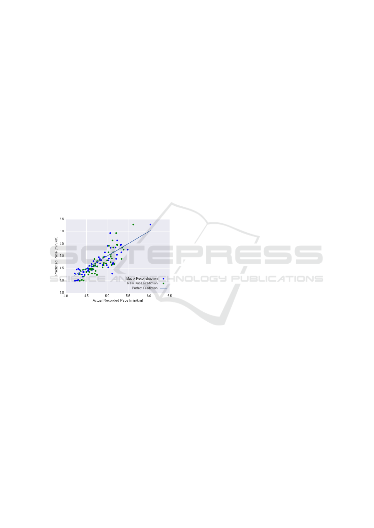
4.2 Results for Predictions on New

Races

Race time prediction accuracy is measured for new

athletes on new races. For this purpose, it is necessary

to know at least N race times for each athlete and that

the routes itinerary is known to compute their features

(distance and cumulative elevation gain).

A few race results can be used to generate ath-

letes vectors using (5) and route features can give race

vectors through the regression model given by (4).

Pace can then be predicted on known races, and com-

pared to actual race records. In this case, race vec-

tors are unknown and are estimated from route prop-

erties. Therefore, the root mean square error increases

to about 26 seconds per kilometer. Figure 4 shows

race pace predictions versus actual records.

Figure 4: Predictions versus observed race times scatter plot

with known vectors or with estimated ones.

5 CONCLUSION

This paper provides tools that can be used to predict

race times. This is of interest for athlete preparation,

for workout route planning and for race events organi-

zation. The same tools can also serve to compare dif-

ferent athlete performances and to track athlete level

over time.

Experiments show that the methodology is appli-

cable to real data and gives meaningful results. This

work will be continued in different directions. First,

only the two most commonly used route features were

used (distance and cumulative positive elevation gain)

but any function of the elevation proﬁle could lead to

better predictive performances. Other route parame-

ters such as ground type and weather conditions may

also prove to improve time prediction.

Then, race vector elements were assumed to be

a linear function of the race features. Other nonlin-

ear regression models could improve the accuracy as

well. Two different approaches can be pursued.

First, domain knowledge was not considered in

this work. Most probably, accuracy could bene-

ﬁt from well-established physiological or empirical

models; for instance, the relationship between aver-

age race pace and distance has been modeled in other

works by hyperbolic law, power law or nomogram

eronnet and Thibault, 1989; Garc

ıa-Manso et al.,

2012; Coquart et al., 2015).

A second path to be taken would be to discover

more complex relationships between route features

and race pace through the data itself using model ﬁt-

ting techniques. This approach will probably require

a larger amount of race data.

REFERENCES

Bauer, C. (2013). On the (in-) accuracy of gps measures

of smartphones: a study of running tracking applica-

tions. In Proceedings of International Conference on

Advances in Mobile Computing & Multimedia, page

335. ACM.

Coquart, J. B., Mercier, D., Tabben, M., and Bosquet, L.

(2015). Inﬂuence of sex and specialty on the predic-

tion of middle-distance running performances using

the mercier et al.s nomogram. Journal of sports sci-

ences, 33(11):1124–1131.

Ekstrand, M. D., Riedl, J., and Konstan, J. A. (2011).

Collaborative ﬁltering recommender systems. Foun-

dations and Trends in Human-Computer Interaction,

4:175–243.

Garc

ıa-Manso, J., Mart

ın-Gonz

alez, J., Vaamonde, D.,

and Da Silva-Grigoletto, M. (2012). The limitations

of scaling laws in the prediction of performance in

endurance events. Journal of theoretical biology,

300:324–329.

Gemulla, R., Nijkamp, E., Haas, P. J., and Sismanis, Y.

(2011). Large-scale matrix factorization with dis-

tributed stochastic gradient descent. In KDD.

Jain, P., Netrapalli, P., and Sanghavi, S. (2013). Low-rank

matrix completion using alternating minimization. In

Proceedings of the forty-ﬁfth annual ACM symposium

on Theory of computing, pages 665–674. ACM.

James, G., Witten, D., Hastie, T., and Tibshirani, R. (2013).

An introduction to statistical learning. volume 112,

chapter 5, pages 176–186. Springer.

Noakes, T. D., Myburgh, K. H., and Schall, R. (1990). Peak

treadmill running velocity during the v o2 max test

predicts running performance. Journal of sports sci-

ences, 8(1):35–45.

eronnet, F. and Thibault, G. (1989). Mathematical analy-

sis of running performance and world running records.

Journal of Applied Physiology, 67(1):453–465.

Riegel, P. S. (1981). Athletic records and human endurance:

A time-vs.-distance equation describing world-record

performances may be used to compare the relative

endurance capabilities of various groups of people.

American Scientist, 69(3):285–290.

ust, C. A., Knechtle, B., Knechtle, P., Barandun, U., Lep-

ers, R., and Rosemann, T. (2011). Predictor variables

for a half marathon race time in recreational male run-

ners. Open access journal of sports medicine, 2:113.

Vickers, A. J. and Vertosick, E. A. (2016). An empiri-

cal study of race times in recreational endurance run-

ners. BMC Sports Science, Medicine and Rehabilita-

tion, 8(1):26.