
The Behavior of Deep Statistical Comparison Approach for Different
Criteria of Comparing Distributions
Tome Eftimov
1,2
, Peter Koro
ˇ
sec
1,3
and Barbara Korou
ˇ
si
´
c Seljak
1
1
Computer Systems Department, Jo
ˇ
zef Stefan Institute, Jamova cesta 39, 1000 Ljubljana, Slovenia
2
Jo
ˇ
zef Stefan International Postgraduate School, Jamova cesta 39, 1000 Ljubljana, Slovenia
3
Faculty of Mathematics, Natural Sciences and Information Technologies, Glagolja
ˇ
ska ulica 8, 6000 Koper, Slovenia
Keywords:
Statistical Comparison, Single Objective Functions, Deep Statistics, Stochastic Optimization Algorithms.
Abstract:
Deep Statistical Comparison (DSC) is a recently proposed approach for the statistical comparison of meta-
heuristic stochastic algorithms for single-objective optimization. The main contribution of the DSC is a rank-
ing scheme, which is based on the whole distribution, instead of using only one statistic, such as average
or median, which are commonly used. Contrary to common approach, the DSC gives more robust statis-
tical results, which are not affected by outliers or misleading ranking scheme. The DSC ranking scheme
uses a statistical test for comparing distributions in order to rank the algorithms. DSC was tested using the
two-sample Kolmogorov-Smirnov (KS) test. However, distributions can be compared using different criteria,
statistical tests. In this paper, we analyze the behavior of the DSC using two different criteria, the two-sample
Kolmogorov-Smirnov (KS) test and the Anderson-Darling (AD) test. Experimental results from benchmark
tests consisting of single-objective problems, show that both criteria behave similarly. However, when algo-
rithms are compared on a single problem, it is better to use the AD test because it is more powerful and can
better detect differences than the KS test when the distributions vary in shift only, in scale only, in symmetry
only, or have the same mean and standard deviation but differ on the tail ends only. This influence is not
emphasized when the approach is used for multiple-problem analysis.
1 INTRODUCTION
Over recent years, many meta-heuristic stochastic op-
timization algorithms have been developed. Perfor-
mance analysis of a new algorithm compared with the
state-of-the-art is a crucial task and one of the most
common ways to compare their performance is to use
statistical tests based on hypothesis testing (Lehmann
et al., 1986). Making, such statistical comparisons,
however, requires sufficient knowledge from the user,
which includes knowing which conditions must be
fulfilled so that the relevant and proper statistical test
(e.g., parametric or nonparametric) can be applied
(Garc
´
ıa et al., 2009).
The nature of stochastic optimization algorithms
means that a set of independent runs must be executed
on a single instance of a problem in order to get a rel-
evant data set over which either average or median
are typically calculated. Further, because the required
conditions (normality and homoscedasticity) for the
safe use of the parametric statistical tests are usually
not satisfied when working with stochastic optimiza-
tion algorithms an appropriate nonparametric statis-
tical test is required. Nonparametric statistical tests
are based on a ranking scheme that is used to trans-
form the data prior to analysis. The standard rank-
ing scheme used by many of the nonparametric sta-
tistical tests ranks the algorithms for each problem
(function) separately with the best performing being
ranked number 1, the second best ranked number 2,
and so on. In case of ties, average rankings are as-
signed. Unfortunately, using either the average or the
median can negatively affect the outcome of the re-
sults of a statistical test (Eftimov et al., 2016). For ex-
ample, averaging is sensitive to outliers, which should
be handled appropriately since stochastic optimiza-
tion algorithms can produce poor runs. For instance,
let us suppose that two algorithms, A
1
and A
2
, are
used to optimize the parabola problem, y = x
2
, and
the results after 10 runs are 0, 0,0,0,0, 0,0, 0,0, 10,
and 0, 1,0, 1,0, 1,0, 1,0, 1, for each algorithm, respec-
tively. We see that the average of A
1
is 1, while the av-
erage of A
2
is 0.5. The standard ranking scheme will
rank, A
1
and A
2
as 2 and 1, respectively. From this,
Eftimov T., KoroÅ ˛aec P. and KorouÅ ˛aiÄ
˘
G Seljak B.
The Behavior of Deep Statistical Comparison Approach for Different Criteria of Comparing Distributions.
DOI: 10.5220/0006499900730082
In Proceedings of the 9th International Joint Conference on Computational Intelligence (IJCCI 2017), pages 73-82
ISBN: 978-989-758-274-5
Copyright
c
2017 by SCITEPRESS – Science and Technology Publications, Lda. All rights reserved

it follows that A
2
is better, but we can see that the al-
gorithm A
1
has only one poor run (outlier), which af-
fects the average. In the case when poor runs are not
present, the average can be in some ε-neighborhood,
which is defined as the set of all numbers whose
distance from a number is less than some specified
number ε, and the algorithms will obtain different
rankings. In order to overcome this problem, medi-
ans are sometimes used because they are more ro-
bust to outliers. However, medians can be in some
ε-neighborhood, and based on these the algorithms
will obtain different rankings. The question is, there-
fore, how to define the ε-neighborhood for different
test problems that have different ranges of obtained
data e.g. 10
−9
, 10
−2
, 10
1
, etc. Let us suppose that
two algorithms, A
1
and A
2
, are new algorithms used
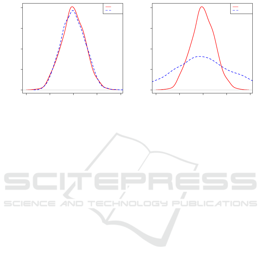
to optimize a given problem, and the results from 100
runs of both algorithms are distributed according to
N(0;1). Figure 1(a), shows the probability density
function of the two algorithms. In this case, the distri-
butions are the same, the median values are in some
ε-neighborhood, and because of this the algorithms
should obtain the same ranking. Now let us sup-
pose that two new algorithms, A
1
and A
2
, are used for
the optimization of a given problem, and the results
from 100 runs are distributed according to N(0; 1) and
N(0;2.5), respectively. Figure 1(b), shows the proba-
bility density function of the two algorithms. In this
case, the distributions are not the same and the me-
dian values are in some ε-neighborhood, and because
of this the algorithms should obtain different rank-
ings. If this is a case, then the algorithms rankings
are obtained either by the averages or the medians,
so the algorithm which has smaller value for aver-
age or median is the better one. For these reasons,
a novel approach was proposed, called Deep Statisti-
cal Comparison (DSC) (Eftimov et al., 2017), which
removes the sensitivity of the simple statistics to the
data and enables calculation of more robust statistics
without fear of outliers influence or some errors inside
ε-neighborhood.
The reminder of the paper is organized as fol-
lows. Section II gives an overview of the related
work, while Section III reintroduces the DSC rank-
ing scheme used to compose a sample of results for
each algorithm for multiple-problem analysis. Sec-
tion IV presents statistical comparisons of stochastic
optimization algorithms over multiple problems. This
is then followed by a discussion of the results. In Sec-
tion V, power analysis of DSC is presented when dif-
ferent statistical tests for comparing distributions are
used in the ranking scheme. The conclusions of the
paper are presented in Section VI.
2 RELATED WORK
Statisticians (Gill, 1999) have shown that researchers
have difficulties performing empirical studies and this
could lead them into misinterpreting their results.
Leven et al. (Levine et al., 2008) also state that the hy-
pothesis testing is also frequently misunderstood and
abused. To select an appropriate statistical test and
to choose between a parametric and a nonparametric
test (Garc
´
ıa et al., 2009), the first step is to check the
assumptions of the parametric tests, in other words,
the required conditions for the safe use of parametric
tests.
Dem
ˇ
sar (Dem
ˇ
sar, 2006) theoretically and empir-
ically examined several suitable statistical tests that
can be used for comparing machine learning algo-
rithms. Following a statistical tutorial on machine
learning algorithms, Garcia et al. (Garc
´
ıa et al.,
2009) presented a study on the use of nonparametric
tests for analyzing the behaviour of evolutionary al-
gorithms for optimization problems. They conducted
their study in two ways: single-problem analysis and
multiple-problem analysis. Single-problem analysis
is a scenario when the data derives from multiple runs
of the stochastic optimization algorithms on one prob-
lem. This scenario is common in stochastic optimiza-
tion algorithms, since they are stochastic in nature,
meaning we do not have any guaranty that the re-
sult will be the same for every run. Even the path
leading to the final solution is often different. To
test the quality of an algorithm, it is not sufficient
to performed just a single run, but many runs are
needed to draw a conclusion. The second scenario,
the multiple-problem analysis, is the scenario when
several stochastic optimization algorithms are com-
pared over multiple problems. In this case, as in most
published papers on this topic, the authors use the av-
erage of the results for each problem in order to pro-
duce results for each algorithm. We call this approach
the “common approach” because it is the one most of-
ten used for making a statistical comparison of meta-
heuristic stochastic optimization algorithms.
Recently, a novel approach for statistical compar-
ison of stochastic optimization algorithms for mul-
tiple single-objective problems was proposed. The
approach is known as Deep Statistical Comparison
(DSC) (Eftimov et al., 2017). The term Deep statis-
tics comes from the ranking scheme that is based on
the whole distribution of multiple runs obtained on a
single problem instead of using some simple statis-
tics such as averages or medians. For this propose,
the DSC was tested using one criteria for comparing
distributions, the two-sample KS test. The approach
consists of two steps, the first step uses a newly pro-
-4 -2 0 2 4
0.0 0.1 0.2 0.3 0.4
-4 -2 0 2 4
Value
Probability density function
N(0,1)
N(0,1)
(a) Same distributions
-4 -2 0 2 4
0.0 0.1 0.2 0.3 0.4
Value
Probability density function
N(0,1)
N(0,2.5)
(b) Different distributions
Figure 1: Probability density functions.
posed ranking scheme to obtain the data that will be
used to make a statistical comparison. The second
step is a standard omnibus statistical test that can be
a parametric or a nonparametric one. DSC approach
also allows users to calculate more robust statistics,
while avoiding wrong conclusions due to either the
presence of outliers or a ranking scheme that is used
in some standard statistical tests.
3 DEEP STATISTICAL
COMPARISON
In this paper, we analyze the behavior of DSC taking
into account different criteria for comparing distribu-
tions used in the DSC ranking scheme. We did this
to see if different criteria for comparing distributions
influence the results from the DSC. The two most
commonly used statistical tests for comparing distri-
butions were selected, the two-sample Kolmogorov-
Smirnov (KS) test and the two-sample Anderson-
Darling (AD) test (Engmann and Cousineau, 2011),
as different criteria for comparing distributions. To
explain this, we start by reintroducing the DSC.
3.1 DSC Ranking Scheme
Let m and k be the number of algorithms and the num-
ber of problems that are used for statistical compari-
son, respectively, and n be the number of runs per-
formed by each algorithm on the same problem.
Let X
i
be a n × m matrix, where i = 1,.. ., k. The
rows of this matrix correspond to the results obtained
by multiple runs on the i-th problem, and the columns
correspond to the different algorithms that are used.
The matrix element X
i
[ j,l], where j = 1,. .. ,n, and
l = 1 .. ., m, corresponds to the result obtained by the
j-th run on the i-th problem of the l-th algorithm.
The ranking scheme is based on the whole distri-
bution, instead of ranking according to the averages
or medians. The first step is to compare the probabil-
ity distributions of multiple runs of each algorithm on
each problem. For this purpose, a statistical test for
comparing distributions should be used. Two most
commonly used tests are the two-sample KS test and
the two-sample AD test.
The two-sample KS test is a nonparametric test
of the equality of continuous, one-dimensional prob-
ability distributions that can be used to compare two
samples. The two-sample KS test is one of the most
useful and general non-parametric methods for com-
paring two samples, as it is sensitive to differences
in both location and shape of the empirical cumula-
tive distribution functions of the two samples (e.g., a
difference with respect to location/central tendency,
dispersion/variability, skewness, and kurtosis) (Sen-
ger and C¸ elik, 2013).
The two-sample AD test has the same advantages
mentioned for the KS test, sensibility to shape and
scale of a distribution and its applicability to small
samples. In addition, it has two extra advantages over
the KS test. First, it is especially sensitive towards
differences at the tails of distributions, and second it
is better capable of detecting very small differences,
even between large sample sizes. More about compar-
ison of the two tests when shift, scale, and symme-
try of distributions are varied independently for dif-
ferent sample sizes can be found in (Engmann and
Cousineau, 2011).

Let α
T
be the significance level used by the statis-
tical test that is selected for comparing distributions.
By using a statistical test for comparing distributions,
m · (m − 1)/2 pairwise comparisons between the al-
gorithms are performed, and the results are organized
into a m × m matrix, M
i
as follows:
M
i
[p,q] =
(
p
value
, p 6= q
1, p = q
, (1)
where p and q are different algorithms and p,q =
1,. .. ,m.
Because multiple pairwise comparisons are made,
this could lead to the family-wise error rate (FWER)
(van der Laan et al., 2004), which is the probability
of making one or more false discoveries, or type I er-
rors, among all hypotheses when performing multiple
hypotheses tests. In the cases when a few algorithms
are compared the influence of multiple comparison in
the FWER may not be very large, but as the num-
ber of compared algorithms increases, the FWER can
increase dramatically. In order to counteract the prob-
lem of multiple comparisons, the Bonferroni correc-
tion (Garc
´
ıa et al., 2010) is used to correct the ob-
tained p-values. The Bonferroni correction is based
on the idea of testing u different hypotheses. One
way of reducing the FWER is to test each individ-
ual hypothesis at a statistical significance level of
1
u
times the desired maximum significance level. In our
case the number of multiple pairwise comparisons,
or the number of different hypotheses, is given as
C
2
m
=
m
2
=
m·(m−1)
2
.
The matrix M
i
is reflexive. Also, it is symmetric
because M
i
= M
T
i
, but the key point for the ranking
scheme is to check the transitivity, since the ranking
is made according to it. For this purpose, the matrix
M
0
i
is introduced using the following equation:
M
0
i
[p,q] =
(
1, M
i
[p,q] ≥ α
T
/C
2
m
0, M
i
[p,q] < α
T
/C
2
m
. (2)
The elements of the matrix, M
0
i
, are defined accord-
ing to the p-values obtained by the statistical test used
for comparing distributions corrected by the Bonfer-
roni correction. For example if the element M
0
i
[p,q] is
1 that means that the null hypothesis used in the sta-
tistical test for comparing distributions, which is the
hypothesis that the two data samples obtained by the
p-th and the q-th algorithm come from the same dis-
tribution, is not rejected. If the element M
0
i
[p,q] is 0
that means that the null hypothesis is rejected, so the
two data samples come from different distributions.
Before the ranking is performed, the matrix M
0
2
i
is
calculated to check the transitivity. If the M
0
i
has a 1
in each position for which M
0
2
i
has non-zero element,
the transitivity is satisfied, otherwise it is not.
If the transitivity is satisfied, the first step is to
split the set of algorithms into w disjoint sets of algo-
rithms Φ
f
, f = 1,...,w, such as each algorithm be-
longs only in one of these sets. Each of these sets
contains the indices of the algorithms that are used in
the comparison for which the transitivity is satisfied.
The cardinality of the union of these sets needs to be
m,
∑
w
f =1
|Φ
f
| = m. The next step is to define a w × 2
matrix, W
i
. The elements of this matrix are defined
with the following equation
W
i
[ f ,x] =
(
mean(Φ
f
{
h
}
), x = 1
|Φ
f
|, x = 2
, (3)
where h is the number that is ceiled to the nearest inte-
ger of a number obtained by the uniform distribution
of a random variable Y ∼ U (1, |Φ
f
|). The algorithm
from each set, whose average value will be used, can
be chosen randomly because the data samples for all
the algorithms that belong to the same set come from
the same distribution. Then the rows of the matrix are
reordered according to the first column sorted in as-
cending order. Let Mean
i
and C be a w × 1 vectors
that correspond to the first and the second column of
the matrix W
i
, respectively. Finally, the rankings to
the sets, Φ
f
, need to be assigned and organized into
a w × 1 vector Rank
s
. For the set with lowest average
value, Mean
i
[1], the ranking is defined as
Rank
s
[1] =
C[1]
∑
r=1
r/C[1]. (4)
For remaining sets, the ranking is defined as
Rank
s
[ f ] =
C[ f −1]+C[ f ]
∑
r=C[ f −1]+1
r/C[ f ]. (5)
After obtaining the rankings of the sets, each algo-
rithm obtains its ranking according to the set to which
it belongs by using the following equation:
Rank[i, l] = Rank
s
[ f ], l ∈ Φ
f
. (6)
If the transitivity is not satisfied, the first step is
to define two 1× m vectors, Index
i
and Mean
i
, whose
elements are the indices of the algorithms and the av-
erage values of the multiple runs for each algorithm.
The both vectors are sorted in ascending order accord-
ing to the average values. Then, the rankings of the
sorted algorithms are organized into a 1 × m vector,
Rank
s
, whose elements are defined with the following
equation.
Rank
s
[l] =
l, ∃! Mean
i
[l] ∈ Mean
i
l
∑
r=l−c+1
r/c, otherwise
,
(7)

where c is the number of elements from Mean
i
that
have value Mean
i
[l]. Finally, the algorithms obtain
their rankings according to the rankings assigned to
their average values by using the following equation:
Rank[i, Index
i
[l]] = Rank
s
[l]. (8)
By using the ranking scheme for the algorithms on
each problem, a k × m matrix, Rank, is defined. The
i-th row of this matrix corresponds to the rankings of
the algorithms obtained by the ranking scheme using
the data samples from the i-th problem. Further, this
matrix is used as input data for statistical comparison
for multiple-problem analysis.
3.2 Selection of a Standard Omnibus
Statistical Test
After ranking the algorithms, the next step is to
choose an appropriate statistical test. The guidelines
on which test to choose are given in (Garc
´
ıa et al.,
2009). Using the new ranking scheme we transformed
only the data that is available for further analysis,
while everything else remain the same.
4 RESULTS AND DISCUSSION
4.1 Black-Box Benchmarking 2015 Test
Functions
To evaluate the behavior of the DSC taking into ac-
count different statistical tests for comparing distribu-
tions, the results from the Black-Box Benchmarking
2015 (BBOB 2015) (Black Box Optimization Com-
petition, ) are used. BBOB 2015 is a competition that
provides single-objective functions for benchmark-
ing. From the competition 15 algorithms are used.
The algorithms used are: BSif (Po
ˇ
s
´
ık and Baudi
ˇ
s,
2015), BSifeg (Po
ˇ
s
´
ık and Baudi
ˇ
s, 2015), BSqi (Po
ˇ
s
´
ık
and Baudi
ˇ
s, 2015), BSrr (Po
ˇ
s
´
ık and Baudi
ˇ
s, 2015),
CMA-CSA (Atamna, 2015), CMA-MSR (Atamna,
2015), CMA-TPA (Atamna, 2015), GP1-CMAES
(Bajer et al., 2015), GP5-CMAES (Bajer et al.,
2015), RAND-2xDefault (Brockhoff et al., 2015),
RF1-CMAES (Bajer et al., 2015), RF5-CMAES (Ba-
jer et al., 2015), Sif (Po
ˇ
s
´
ık and Baudi
ˇ
s, 2015), Sifeg
(Po
ˇ
s
´
ık and Baudi
ˇ
s, 2015), and Srr (Po
ˇ
s
´
ık and Baudi
ˇ
s,
2015). For each of them results for 22 different noise-
less test problems in 5 dimensionality (2, 3, 5, 10, and
20) are selected. More details about test problems can
be found in (Hansen et al., 2010). Each algorithm pro-
vided data for 15 runs.
4.2 Experiments
Let Ψ be the set of the selected 15 stochastic opti-
mization algorithms. For the experiments, the dimen-
sion is fixed to 10. A 100 random combinations of
3 distinct algorithms were generated (combinations
without repetition) and used for statistical compar-
isons.
For each combination, the DSC ranking scheme
is used to rank the algorithms for each problem sep-
arately. To compare the results using different cri-
teria for comparing distributions, the DSC ranking
scheme is used with the two-sample KS test and the
two-sample AD test. Then, the results are also com-
pared with the common approach, for which a sample
of results for each algorithm is composed by averag-
ing the data from multiple runs for each problem.
After obtaining the data for statistical comparison
over multiple problems, the next step is to select an
appropriate statistical test. In the case of the DSC
the significance level for the ranking scheme is set to
α
T
= 0.05, and the significance level for the statistical
test is set to α = 0.05.
Table 1 presents the p-values obtained for 6 com-
binations out of 100 generated, using the two versions
of DSC approach, by using the KS test and the AD
test, and the common approach with averages. The
p
value
F
corresponds to the p-values obtained by the
Friedman test, which in our case is one of the appro-
priate omnibus statistical tests. From this table, we
can see that the results for the first 2 combinations (1-
2) differ. By using the common approach with aver-
ages, the null hypothesis is rejected, so there is signif-
icant statistical difference between the performance
of the algorithms, while with both versions of DSC
approach, the null hypothesis is not rejected, so we
can assume that there is no significant statistical dif-
ference between the performance of the algorithms.
The number of such combinations in our experiment
is 5 out of 100. For the next 2 combinations (3-4), the
common approach and both DSC versions give the
same results, the p-values obtained are greater than
0.05, so the null hypothesis is not rejected, and we can
assume that there is no significant statistical differ-
ence between the performance of the algorithms. The
number of such combinations in our experiment is 9
out of 100, from which 2 randomly selected are pre-
sented in the table. For the last 2 combinations from
this table (5-6), the results obtained are the same, the
p-values are smaller than the significance level used,
so the null hypothesis is rejected, and we can assume
that there is a significant statistical difference between
the performance of the algorithms. The number of
such combinations in our experiment is 86 out of 100,

from which 2 are randomly selected and presented in
the table.
In order to explain the difference that appears us-
ing the common approach and the two versions of the
DSC, one example where the result from the common
approach and both versions of the DSC differs is ran-
domly selected and presented in detail. The first com-
bination from the Table 1 is selected, which is a com-
parison between the algorithms GP5-CMAES, Sifeg,
and BSif. For the analysis, the Friedman test was se-
lected. In the case of the common approach, the null
hypothesis is rejected, while when the DSC approach
is used, the null hypothesis is not rejected. The rank-
ings obtained by the Friedman test using the common
approach with averages and both versions of the DSC
ranking scheme are presented in Table 2. Comparing
the rankings obtained by the common approach and
the DSC ranking scheme, the difference between the
rankings that appears by using them can be clearly ob-
served. To explain the difference, separate problems
are discussed in detail.
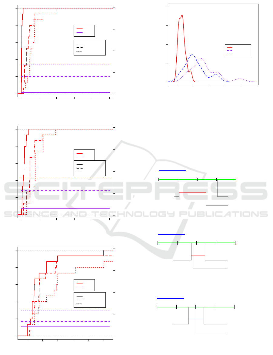
In Figure 2 the cumulative distributions (the step
functions) and the average values (the horizontal
lines) obtained from the multiple runs for different
functions of the three algorithms are presented. In
this figure details about the function, f
7
, are pre-
sented. The rankings obtained using the common ap-
proach with averages are 1.00, 2.00, and 3.00, and
they are different because all of them have different
averages. The rankings obtained using the two ver-
sions of DSC ranking scheme, by using KS test and
AD test, are 1.00, 2.50, and 2.50. The DSC ranking
scheme used the cumulative distributions in order to
assign the rankings of the algorithms. From the fig-
ure, one may assume that there is no significant dif-
ference between the cumulative distributions of Sifeg
and BSif, but they differ from the cumulative distribu-
tion of GP5-CMAES. This result is also obtained by
using the two-sample KS and AD test. The p-values
obtained for the pairs of algorithms are 0.00 (GP5-
CMAES, Sifeg), 0.00 (GP5-CMAES, BSif), and 0.07
(Sifeg, BSif), by using the KS test, while the p-values
obtained for the same pairs of algorithms by using the
AD test are 0.00 (GP5-CMAES, Sifeg), 0.00 (GP5-
CMAES, BSif), and 0.02 (Sifeg, BSif). Because mul-
tiple pairwise comparisons are made, these p-values
are further corrected by using the Bonfferoni correc-
tion. In this case, the transitivity of the matrix M
7
0
is
satisfied, so the set of all algorithms is split into two
disjoint sets {GP5-CMAES}, and {Sifeg, BSif}, and
the rankings are defined using Equations 4 and 5.
In Figure 2(c) the results for the function, f
21
,
are presented. The rankings obtained using the com-
mon approach with averages are 1.00, 2.00, and 3.00,
and they are different because all of them have differ-
ent average. The rankings obtained using the DSC
ranking scheme by using the KS test and AD test
are 2.00, 2.00, and 2.00. From the figure, it is not
clear if there is a significant difference between the
cumulative distributions of GP5-CMAES, Sifeg, and
BSif. To check this, the two-sample KS test and
AD test are used. The p-values obtained for the
pairs of algorithms are 0.38 (GP5-CMAES, Sifeg),
0.07 (GP5-CMAES, BSif), and 0.38 (Sifeg, BSif),
and 0.41 (GP5-CMAES, Sifeg), 0.02 (GP5-CMAES,
BSif), and 0.29 (Sifeg, BSif), respectively. Because
multiple pairwise comparisons are made, these p-
values are further corrected using the Bonfferoni cor-
rection. In this case, the transitivity of the matrix M
21
0
is satisfied, but the set of all algorithms is not split into
disjoint sets because all algorithms belong to one set,
{GP5-CMAES, Sifeg, BSif}.
In Figure 2(b), the results for the function, f
18
, are
presented. This example is interesting because both
versions of the DSC ranking scheme that use differ-
ent criteria for comparing distributions, the KS test
and AD test, give different results. For the function
f
18
, the rankings obtained by the common approach
are 1.00, 2.00, and 3.00. The rankings obtained by
the DSC ranking scheme with KS test are 1.00, 2.50,
and 2.50, while the AD test are 1.00, 2.00, and 3.00.
So the two different criteria used by the DSC rank-
ing scheme give different results. The p-values ob-
tained by using the KS test for the pairs of algorithms
are 0.00 (GP5-CMAES, Sifeg), 0.00 (GP5-CMAES,
BSif), and 0.03 (Sifeg, BSif). Because multiple pair-
wise comparisons are made, these p-values are further
corrected by using the Bonfferoni correction. In this
case, the transitivity of the matrix M
18
0
is satisfied, so
the set of all algorithms is split into two disjoint sets
{GP5-CMAES}, and {Sifeg, BSif}. The p-values ob-
tained by using the AD test for the pairs of algorithms
are 0.00 (GP5-CMAES, Sifeg), 0.00 (GP5-CMAES,
BSif), and 0.01 (Sifeg, BSif). Because multiple pair-
wise comparisons are made, these p-values are further
corrected using Bonfferoni correction. In this case,
the transitivity of the matrix M
18
0
is not satisfied, so
the algorithms obtain their rankings according to their
averages. So, the two different criteria give different
results. This result is important when we compare al-
gorithms on one problem (function), while it does not
influence the result when we are performing multiple-
problem analysis. Even more, when we are compar-
ing algorithms on one problem, it is better to use AD
test because it is more powerful and it can better de-
tect differences than the KS test when the distributions
vary in shift only, in scale only, in symmetry only, or
that have the same mean and standard deviation but

Table 1: Statistical comparisons of 3 algorithms.
Algorithms
Common approach DSC approach (KS) DSC approach (AD)
p
value
F
p
value
F
p
value
F
1 GP5-CMAES, Sifeg, BSif
*
(.02) (.42) (.44)
2 BSif, RF1.CMAES, Sifeg
*
(.00) (.28) (.33)
3 BSifeg, RF1-CMAES, BSrr (.16) (.28) (.48)
4 Sif, Bsrr, GP1-CMAES (.35) (.77) (.83)
5 BSifeg, GP1-CMAES, CMA-CSA
∗
(.00)
∗
(.00)
∗
(.00)
6 BSrr, RAND-2xDefault, Srr
∗
(.00)
∗
(.00)
∗
(.00)
*
indicates that the null hypothesis is rejected, using α = 0.05
p
value
F
corresponds to the p-value obtained by the Friedman test
Table 2: Rankings for the algorithms A
1
=GP5-CMAES, A
2
=Sifeg, and A
3
=BSif.
F
Common approach
(Friedman test)
DSC ranking
scheme (KS test)
DSC ranking
scheme (AD test)
A
1
A
2
A
3
A
1
A
2
A
3
A
1
A
2
A
3
f
1
3.00 2.00 1.00 3.00 2.00 1.00 3.00 2.00 1.00
f
2
3.00 2.00 1.00 3.00 2.00 1.00 3.00 2.00 1.00
f
3
13.00 2.00 1.00 3.00 2.00 1.00 3.00 2.00 1.00
f
4
3.00 1.00 2.00 3.00 1.00 2.00 3.00 1.00 2.00
f
5
3.00 1.50 1.50 2.00 2.00 2.00 2.00 2.00 2.00
f
6
3.00 1.00 2.00 3.00 1.00 2.00 2.50 1.00 2.50
f
7
1.00 2.00 3.00 1.00 2.50 2.50 1.00 2.50 2.50
f
8
3.00 1.00 2.00 3.00 1.50 1.50 3.00 1.00 2.00
f
9
3.00 1.00 2.00 3.00 1.50 1.50 3.00 1.50 1.50
f
10
1.00 2.00 3.00 1.00 2.50 2.50 1.00 2.50 2.50
f
11
1.00 2.00 3.00 1.00 2.50 2.50 1.00 2.50 2.50
f
12
3.00 2.00 1.00 3.00 1.50 1.50 3.00 1.50 1.50
f
13
2.00 1.00 3.00 1.50 1.50 3.00 1.50 1.50 3.00
f
14
3.00 1.00 2.00 2.50 2.50 1.00 2.50 2.50 1.00
f
15
2.00 1.00 3.00 2.00 2.00 2.00 2.00 2.00 2.00
f
16
2.00 1.00 3.00 2.00 2.00 2.00 2.00 1.00 3.00
f
17
1.00 2.00 3.00 1.00 2.50 2.50 1.00 2.50 2.50
f
18
1.00 2.00 3.00 1.00 2.50 2.50 1.00 2.00 3.00
f
19
3.00 1.00 2.00 3.00 1.50 1.50 3.00 1.50 1.50
f
20
3.00 1.00 2.00 3.00 1.50 1.50 3.00 1.50 1.50
f
21
1.00 2.00 3.00 2.00 2.00 2.00 2.00 2.00 2.00
f
22
1.00 2.00 3.00 2.00 2.00 2.00 2.00 2.00 2.00
differ on the tail ends only (Engmann and Cousineau,
2011). Also, it requires less data than the KS test to
reach sufficient statistical power. To see this differ-
ence, in Figure 3 the probability density functions for
the data of each algorithm obtained on the function
f
18
are presented. From it, we can see that the KS test
can not detect the small differences that exist between
the probability distributions of the algorithms Sifeg
and BSif, but the AD test can detect them.
If the null hypothesis is rejected by an omnibus
statistical test, an appropriate post-hoc test should be
used (Dem
ˇ
sar, 2006; Garc
´
ıa et al., 2009). Post-hoc
tests are not a subject in this paper because we ana-
lyze the behavior of a ranking scheme that can be used
for omnibus statistical tests. However, one of them is
used to show differences that exist in the case of the
common approach and the DSC approach. Since we
are interested to compare all algorithms to each other,
we decided to use the Nemenyi test (Nemenyi, 1963),
which is an appropriate post-hoc test for the Friedman
0 20 40 60 80 100
0.0 0.2 0.4 0.6 0.8 1.0
Value
Cumulative distirbution
0 10 20 30 40
Mean
GP5-CMAES
Sifeg
BSif
DSC
mean
(a) f
7
0 20 40 60 80 100
0.0 0.2 0.4 0.6 0.8 1.0
Value
Cumulative distirbution
0 10 20 30 40
Mean
GP5-CMAES
Sifeg
BSif
DSC
mean
(b) f
18
0 5 10 15 20 25
0.0 0.2 0.4 0.6 0.8 1.0
Value
Cumulative distirbution
0 10 20 30 40
Mean
GP5-CMAES
Sifeg
BSif
DSC
mean
(c) f
21
Figure 2: Cumulative distributions (the step functions) and
mean values (the horizontal lines) for different functions of
GP5-CMAES, Sifeg, and BSif.
0 10 20 30 40 50
0.00 0.05 0.10 0.15 0.20
Value
Probability density function
GP5-CMAES
Sifeg
BSif
Figure 3: Probability density functions for f
18
for the algo-
rithms GP5-CMAES, Sifeg, and BSif.
test. In Figure 4, the results obtained by the Nemenyi
test are presented for the common approach with av-
erages and both versions of DSC approach. When
comparing all the algorithms against each other, the
groups of algorithms that are not significantly differ-
ent are connected together.
CD=0.71
1.0
GP5-CMAES
Sifeg
BSif
1.5 2.0 2.5 3
(a) Comparison of all algorithms against each other with the
Nemenyi test (common approach using averages).
CD=0.71
1.0
Sifeg
BSif GP5-CMAES
1.5 2.0 2.5 3
(b) Comparison of all algorithms against each other with the
Nemenyi test (DSC approach with KS test).
CD=0.71
1.0
GP5-CMAES
BSif
Sifeg
1.5 2.0 2.5 3
(c) Comparison of all algorithms against each other with the
Nemenyi test (DSC approach with AD test).
Figure 4: Visualization of post-hoc tests used for the algo-
rithms GP5-CMAES, Sifeg, and BSif.
5 POWER ANALYSIS
The power of a statistical test is defined as the proba-
bility that the test will (correctly) reject the false null
hypothesis. The comparison of the statistical power
of the two-sample KS test and the two-sample AD test
is presented in (Engmann and Cousineau, 2011). The
comparison of the statistical power between the DSC
and the common approach is presented in (Eftimov
et al., 2017). Here we focus on power analysis be-
tween the two versions of the DSC approach that use
different criteria for comparing distributions. For this
purpose the power analysis is presented through an
experimental analysis introduced in (Dem
ˇ
sar, 2006).
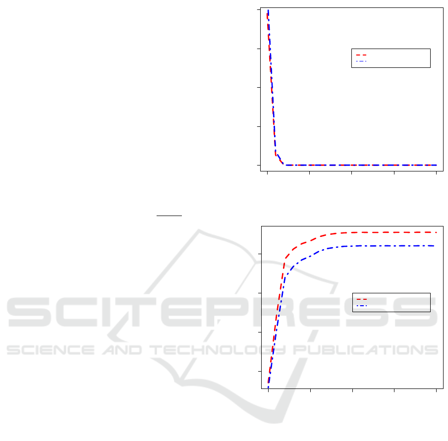
The experimental analysis of the power is made by
a Monte-Carlo simulation. When we are comparing
algorithms, samples of ten problems (functions) were
randomly selected so that the probability for the prob-
lem i being chosen was proportional to
1
1+e
−kd
i
, where
d
i
is the difference between the rankings of the algo-
rithms that are randomly chosen on that problem and
k is the bias through which we can regulate the dif-
ferences between the algorithms. Figure 5(a) repre-
sents the number of hypotheses rejected between the
three algorithms considered with a significance level
of 0.05 and Figure 5(b) represents their associated av-
erage p-values. From them, we can conclude that both
versions of DSC approach behave similarly. The two-
sample AD test has better power than the two-sample
KS test (Engmann and Cousineau, 2011), but this in-
fluence is not emphasized in the case of the DSC ap-
proach.
6 CONCLUSION
We analyze the behavior of the deep statistical com-
parison (DSC) approach taking into account differ-
ent criteria for comparing distributions. The approach
consists of two steps. In the first step, a new ranking
scheme is used to obtained data for mulitple-problem
analysis. The ranking scheme is based on comparing
distributions, instead of using simple statistics such
as averages or medians. The second step is a stan-
dard omnibus statistical test, which uses the data ob-
tained by the DSC ranking scheme as input data. By
using the DSC, the wrong conclusions caused by the
presence of outliers or ranking scheme used by some
standard statistical tests can be avoided.
In this paper, different criteria for comparing dis-
tributions were used in the DSC ranking scheme, to
see if there is a difference between the obtained re-
sults. We used two criteria for comparing distri-
butions, the two-sample Kolmogorov-Smirnov (KS)
0 5 10 15 20
0 100 200 300 400
k
Number of hypotheses rejected
DSC approach (KS test)
DSC approach (AD test)
(a) Number of hypotheses rejected
0 5 10 15 20
0.2 0.4 0.6 0.8
k
Average p-value
DSC approach (KS test)
DSC approach (AD test)
(b) Average p-value
Figure 5: Power analysis for the combination CMA-MSR,
Sifeg, and BSifeg.
test and the two-sample Anderson-Darling (AD) test.
From the experimental results obtained over the al-
gorithms presented in the BBOB 2015, we can con-
clude that both versions of DSC approach behave sim-
ilarly. However, when we are comparing algorithms
on one problem, it is better to use AD test because it
is more powerful and it can better detect differences
than the KS test when the distributions vary in shift
only, in scale only, in symmetry only, or have the
same mean and standard deviation but differ on the
tail ends only (Engmann and Cousineau, 2011). Also,
it requires less data than the KS test to reach sufficient
statistical power. The two-sample AD test has better
power than the two-sample KS test, but this influence

is not emphasized when the DSC approach is used for
multiple-problem analysis.
ACKNOWLEDGEMENTS
This work was supported by the project ISO-FOOD,
which received funding from the European Union’s
Seventh Framework Programme for research, techno-
logical development and demonstration under grant
agreement no 621329 (2014-2019) and the project
that has received funding from the Slovenian Re-
search Agency (research core funding No. L3-7538).
REFERENCES
Atamna, A. (2015). Benchmarking ipop-cma-es-tpa and
ipop-cma-es-msr on the bbob noiseless testbed. In
Proceedings of the Companion Publication of the
2015 on Genetic and Evolutionary Computation Con-
ference, pages 1135–1142. ACM.
Bajer, L., Pitra, Z., and Hole
ˇ
na, M. (2015). Benchmark-
ing gaussian processes and random forests surrogate
models on the bbob noiseless testbed. In Proceed-
ings of the Companion Publication of the 2015 on
Genetic and Evolutionary Computation Conference,
pages 1143–1150. ACM.
Black Box Optimization Competition, B. Black-
box benchmarking 2015. http://coco.gforge.inria.fr/
doku.php?id=bbob-2015. Accessed: 2016-02-01.
Brockhoff, D., Bischl, B., and Wagner, T. (2015). The
impact of initial designs on the performance of mat-
sumoto on the noiseless bbob-2015 testbed: A prelim-
inary study. In Proceedings of the Companion Publi-
cation of the 2015 on Genetic and Evolutionary Com-
putation Conference, pages 1159–1166. ACM.
Dem
ˇ
sar, J. (2006). Statistical comparisons of classifiers
over multiple data sets. The Journal of Machine
Learning Research, 7:1–30.
Eftimov, T., Koro
ˇ
sec, P., and Korou
ˇ
si
´
c Seljak, B. (2016).
Disadvantages of statistical comparison of stochastic
optimization algorithms. In Proceedings of the Bioin-
spired Optimizaiton Methods and their Applications,
BIOMA 2016, pages 105–118. JSI.
Eftimov, T., Koro
ˇ
sec, P., and Seljak, B. K. (2017). A novel
approach to statistical comparison of meta-heuristic
stochastic optimization algorithms using deep statis-
tics. Information Sciences, 417:186–215.
Engmann, S. and Cousineau, D. (2011). Comparing dis-
tributions: the two-sample anderson-darling test as an
alternative to the kolmogorov-smirnoff test. Journal
of Applied Quantitative Methods, 6(3):1–17.
Garc
´
ıa, S., Fern
´
andez, A., Luengo, J., and Herrera, F.
(2010). Advanced nonparametric tests for multi-
ple comparisons in the design of experiments in
computational intelligence and data mining: Exper-
imental analysis of power. Information Sciences,
180(10):2044–2064.
Garc
´
ıa, S., Molina, D., Lozano, M., and Herrera, F. (2009).
A study on the use of non-parametric tests for ana-
lyzing the evolutionary algorithms behaviour: a case
study on the cec2005 special session on real parameter
optimization. Journal of Heuristics, 15(6):617–644.
Gill, J. (1999). The insignificance of null hypothesis
significance testing. Political Research Quarterly,
52(3):647–674.
Hansen, N., Auger, A., Finck, S., and Ros, R. (2010).
Real-parameter black-box optimization benchmark-
ing 2010: Experimental setup.
Lehmann, E. L., Romano, J. P., and Casella, G. (1986). Test-
ing statistical hypotheses, volume 150. Wiley New
York et al.
Levine, T. R., Weber, R., Hullett, C., Park, H. S., and Lind-
sey, L. L. M. (2008). A critical assessment of null
hypothesis significance testing in quantitative commu-
nication research. Human Communication Research,
34(2):171–187.
Nemenyi, P. (1963). Distribution-free multiple compar-
isons. In PhD Thesis. Princeton University.
Po
ˇ
s
´
ık, P. and Baudi
ˇ
s, P. (2015). Dimension selection in
axis-parallel brent-step method for black-box opti-
mization of separable continuous functions. In Pro-
ceedings of the Companion Publication of the 2015 on
Genetic and Evolutionary Computation Conference,
pages 1151–1158. ACM.
Senger,
¨
O. and C¸ elik, A. K. (2013). A monte carlo
simulation study for kolmogorov-smirnov two-sample
test under the precondition of heterogeneity: upon
the changes on the probabilities of statistical power
and type i error rates with respect to skewness mea-
sure. Journal of Statistical and Econometric Methods,
2(4):1–16.
van der Laan, M. J., Dudoit, S., and Pollard, K. S. (2004).
Multiple testing. part ii. step-down procedures for
control of the family-wise error rate. Statistical appli-
cations in genetics and molecular biology, 3(1):1–33.
