R-FCN Object Detection Ensemble based on Object Resolution and

Image Quality

Christoffer Bøgelund Rasmussen, Kamal Nasrollahi and Thomas B. Moeslund

Visual Analysis of People (VAP) Laboratory, Aalborg University, Aalborg, Denmark

Keywords:

Convolutional Neural Networks, Object Detection, Image Quality Assessment, Ensemble Learning.

Abstract:

Object detection can be difﬁcult due to challenges such as variations in objects both inter- and intra-class. Ad-

ditionally, variations can also be present between images. Based on this, research was conducted into creating

an ensemble of Region-based Fully Convolutional Networks (R-FCN) object detectors. Ensemble strategies

explored were ﬁrstly data sampling and selection and secondly combination strategies. Data sampling and se-

lection aimed to create different subsets of data with respect to object size and image quality such that expert

R-FCN ensemble members could be trained. Two combination strategies were explored for combining the

individual member detections into an ensemble result, namely average and a weighted average. R-FCNs were

trained and tested on the PASCAL VOC benchmark object detection dataset. Results proved positive with an

increase in Average Precision (AP), compared to state-of-the-art similar systems, when ensemble members

were combined appropriately.

1 INTRODUCTION

Object detection is a fundamental area of computer

vision that has had a great amount of research over

the past decades. The general goal of object detec-

tion is to ﬁnd a speciﬁc object in an image. The spe-

ciﬁc object is typically from a pre-deﬁned list of cate-

gories that are of interest. Object detection generally

consists of two larger tasks; localisation and classiﬁ-

cation. Localisation is typically drawing a bounding-

box around the object indicating where a given object

is in the image and classiﬁcation is determining the

type of the object with an associated conﬁdence.

Object detection is a challenging problem due to

both large scale issues and minute differences be-

tween objects. Firstly, there is the challenge of

differentiating objects between classes. Depending

on the problem at hand the number of potential

classes present can be thousands or tens of thou-

sand. On top of this, separate object categories

can be both very different in appearance, for ex-

ample an apple and an aeroplane, but separate cat-

egories can also be similar in appearance, such as

dogs and wolves. These main challenges of object

detection stem from two categories which deﬁned

per (Zhang et al., 2013) as: robustness-related and

computational-complexitity and scalability-related.

Robustness-related refers to the challenges in ap-

pearance variations within the both of intra-class and

inter-class. These variations can be categorised into

two types as per (Schroff, 2009) as: object and image

variations. Object variations consist of appearance

differences between object instances with respect to

factors such as colour, texture, shape, and size. Image

variations are differences not related to the object in-

stances themselves but rather the actual image. This

can consist of conditions such as lighting, viewpoint,

scale, occlusion, and clutter. Based upon these dif-

ferences the task of both classifying a given object

as a given class but also differentiating the potentially

largely varying objects into the same class is challeng-

ing.

Current state-of-the-art in object detection is

within the realm of deep learning with Convolutional

Neural Networks (CNN)s. Deep learning methods are

of such a scale that given appropriate data have been

able to address the two main challenges mentioned

earlier. This is exempliﬁed with almost all leading en-

tries in benchmark challenges such as PASCAL VOC

(Everingham et al., 2010), ImageNet (Russakovsky

et al., 2015), and MSCOCO (Lin et al., 2014) con-

sisting of CNN-based approaches. Additionally, re-

cent trends with CNN-based object detection methods

have been to incorporate ensembles of networks to

further enhance performance (He et al., 2015) (Huang

et al., 2016) (Li et al., 2016).

Rasmussen C., Nasrollahi K. and Moeslund T.

R-FCN Object Detection Ensemble based on Object Resolution and Image Quality.

DOI: 10.5220/0006511301100120

In Proceedings of the 9th International Joint Conference on Computational Intelligence (IJCCI 2017), pages 110-120

ISBN: 978-989-758-274-5

One of the main goals of an ensemble system is to

reduce the variance incorporated in the training pro-

cess. An example is to train classiﬁers on different

subsets of the data, creating a number of different en-

semble members. The assumption is that the classi-

ﬁers will make different errors on a given data point.

However, by combining the classiﬁers the errors will

be mitigated by the increased strength from lower in-

dividual variance. The ensemble members created

in this work address two of the three main strategies

from (Zhang and Ma, 2012) to build an ensemble sys-

tem. Namely:

1. Data sampling and selection: selection of training

data for individual classiﬁers.

2. Training member classiﬁers: speciﬁc procedure

used for generating ensemble members.

3. Combining ensemble members: combination rule

for obtaining ensemble decision.

The robustness-related challenges are addressed

by exploring the possibilities of designing expert en-

semble members towards both object and image vari-

ations in a leading object detection benchmark. This

is done by training an ensemble of Region-based

Fully Convolutional Network (R-FCN) with ResNet-

101 networks. Data sampling strategies are used to

create subsets of data with respect to object resolution

and various image quality factors. Finally, two sepa-

rate combination strategies are explored for combin-

ing the ensemble members. The rest of this paper is

organized as follows: the related works are reviewed

in the next section.

2 RELATED WORK

One of the ﬁrst methods to show that CNN could

signiﬁcantly improve object detection was that of R-

CNN (Girshick et al., 2014). The method obtains

the name R-CNN as a Convolutional Neural Network

(CNN) is used on regions of the image. Regions are

pre-computed as proposals using a method such as

SelectiveSearch (Uijlings et al., 2013) to give an in-

dication as to where objects may be located. In R-

CNN the CNN model is used as a feature extractor

from which a class-speciﬁc linear Support Vector Ma-

chine (SVM) can be trained on top of. The AlexNet-

based feature extractor is ﬁrstly pre-trained on a large

dataset designed for classiﬁcation and then ﬁne-tuned

to object detection. Each pre-computed region pro-

posal is run through a forward pass of the model to

extract features and then passed to the SVM.

The R-CNN method was improved the following

year with Fast R-CNN (Girshick, 2015) and aimed

to improve speed and accuracy. One of the signif-

icant changes is that training end-end rather than in

the multi-stage pipeline in R-CNN. A CNN is again

used as a feature extractor where Region of Interest

(RoI) pooling is conducted on the ﬁnal feature map.

Afterwards the forward pass continues through two

fully-connected layers followed by two sibling output

layers replacing the external SVM. The sibling out-

puts are a softmax classiﬁcation layer that produces

probabilities for the object classes and another layer

for bounding-box regression. In R-CNN, the only

deep network used was AlexNet (Krizhevsky et al.,

2012), however, in Fast R-CNN the authors experi-

ment with networks of different size. It was found

that the deeper network VGG-16 (Simonyan and Zis-

serman, 2015) for computing the convolutional fea-

ture map gave a considerable improvement in perfor-

mance. As the name implies the main improvement is

the speed in respect to both training and testing. By

computing a convolutional feature map for an entire

image rather than per object proposal the number of

passes in the network is lowered signiﬁcantly. While

Fast R-CNN provided improvements in both accuracy

and speed, the increase in speed is only in relation to

the actual object detection and assumes that the region

proposals are pre-computed. Therefore, there is still a

signiﬁcant bottleneck per image as a region proposal

method can typically take a couple of seconds.

Faster R-CNN (Ren et al., 2015) addressed this

bottleneck in the third iteration of the R-CNN method.

Faster R-CNN showed that region proposals could be

computed as part of the network through the use of a

Region Proposal Network (RPN). The RPN shares the

convolutional layers and feature map used for com-

puting features with RoI pooling in Fast R-CNN. As

these layers are already computed on the entire im-

age for the classiﬁcation pipeline, the added time for

proposals using the RPN is negligible. Apart from the

change in how region proposals are computed, there is

no difference in comparison to Fast R-CNN. An RPN

takes the last convolutional feature map as input and

returns a number of object proposals.

The winner of the Microsoft Common Objects in

Context (MS COCO) 2015 and ImageNet Large Scale

Visual Recognition Challenge (ILSVRC) 2015 detec-

tion challenge was based on deep residual networks

(ResNets) (He et al., 2015). As is well known with

CNNs, deeper networks are able to capture richer

higher-level features. The authors showed that this is

also beneﬁcial in the object detection domain. In (He

et al., 2015) an ensemble of three deep residual net-

works with 101 layers was trained for object detection

and another ensemble of three used for region pro-

posals with the RPN while being based on the Faster

R-CNN framework. In addition to the ensemble, the

winning entry also added box reﬁnement, global con-

text, and multi-scale testing to the Faster R-CNN.

The current leading method on MS COCO is an

extension of the previously explained ResNets (He

et al., 2015). This method denoted as G-RMI on the

MS COCO leaderboard (COCO, 2017) is an ensem-

ble of ﬁve deep residual networks based upon ResNet

(He et al., 2015) and Inception ResNet (Szegedy et al.,

2016) feature extractors. No work has been published

yet on G-RMI at this time, however, a short explana-

tion of the entry is included in a survey paper from the

winning authors (Huang et al., 2016). The approach

was to train a large number of Faster R-CNN mod-

els with varying output stride, variations on the loss

function, and different ordering of the training data.

Based upon the collection of models, ﬁve were greed-

ily chosen based upon performance on a validation

set. While performance on the models were impor-

tant, the models were also chosen such that they were

not too similar.

Recently, a newer approach to region-based meth-

ods has been proposed with the use of Fully Convo-

lutional Networks (FCNs) through the R-FCN (Dai

et al., 2016). The overall approach is similar to that

used in region-based methods such as (Girshick et al.,

2014), (Girshick, 2015) and (Ren et al., 2015). First,

it computes region proposals using a region proposal

method and then it performs a classiﬁcation on these

regions. R-FCN uses the RPN from Faster R-CNN

(Ren et al., 2015) for proposal computation. However,

RoI pooling is performed on position sensitive score

maps rather than the last feature map. The score maps

are split up to represent a relative position in a k × k

grid, with each cell presenting information relative to

the spatial position of an object.

3 OBJECT DETECTION WITH

R-FCN

One of the current leading object detection methods is

the R-FCN (Dai et al., 2016). The authors of R-FCN

were inspired by the recent advances in FCN classiﬁ-

cation networks. R-FCN uses position-sensitive score

maps computed by a bank of convolutional layers.

The maps add translation variance into the detection

pipeline by computing scores in relation to position

information with respect to the relative spatial posi-

tion of an object. A RoI-pooling layer is added after

the score-maps, however, no convolutional operations

are done after this point ensuring translation variance.

The overall approach of the R-FCN also con-

sists of the popular two-stages of region proposal and

region classiﬁcation. Region proposal is done us-

ing the RPN from Faster R-CNN followed by the

position-sensitive score maps and RoI pooling for re-

gion classiﬁcation. Similar to Faster R-CNN, convo-

lutional layers are applied on the input image and the

RPN computes region proposals. After this, position-

sensitive score maps aid in classiﬁcation.

The added translation variance post ﬁnding pro-

posals with the RPN by producing a bank of k

score

maps for each object category. Therefore, there are

a total of k

(C + 1) maps. The number of k

maps

is due to a k × k spatial grid representing relative po-

sitions. Typically k = 3, therefore, nine score maps

represent position-sensitive scores for a given object

category. For a given RoI placement the vote for rel-

ative position is sampled from their respective map in

the bank.

Once the bank of score maps have been com-

puted, position-sensitive RoI-pooling is found for re-

gion classiﬁcation. Each individual k × k bin pools

from its corresponding location in the relevant score

map. For example, the top left bin pools from that

position in the top-left score map and so on. The

ﬁnal decision for a given class is determined by a

vote where each of the bins are averaged, producing a

(C +1)-dimensional vector for each RoI.

4 PROPOSED METHOD

An ensemble of R-FCNs with the ResNet-101 model

will be trained towards different robustness-related

challenges in the Pattern Analysis, Statistical Mod-

elling and Computational Learning Visual Object

Classes (PASCAL VOC) dataset. The data used will

follow the leading methods for PASCAL VOC 2007

object detection. Training will be done on the 07+12

train sets and testing was conducted on the 07 test set.

Evaluation was conducted using the Average Preci-

sion (AP) metric as per the 07 guidelines.

Leading object detection systems take advantage

of ensemble methods. Many of them are trained with

regards to the variations in internal architecture and

not speciﬁcally training experts towards solving spe-

ciﬁc challenges. Therefore, the system in this work

will take advantage of the ﬁrst ensemble strategy from

(Zhang et al., 2013), data sampling and selection. The

individual R-FCNs were trained on different subsets

of training data with the aim to create expert ensem-

ble members in regards robustness-related challenges,

namely object resolution and image quality.

The third strategy in building an ensemble system,

to combine predictions from individual members of

the ensemble is also addressed. Bounding-boxes and

the conﬁdence of each detection will be combined us-

ing an averaging and a weighted averaging method is

tested on a number of different combinations of en-

semble members.

4.1 Training Ensemble Members

The training of the R-FCN members will be done us-

ing Convolutional Architecture for Fast Feature Em-

bedding (Caffe) (Jia et al., 2014). This was chosen

due to the research being available from the authors

of R-FCN through training code and pre-trained Caffe

models. As there is the requirement to combine de-

tections between ensemble members, the detections

must be found based upon the same input to each

model. This is ensured by using pre-computed re-

gion proposals found using an RPN. In a standard R-

FCN the RPN is an internal part of the network and

is trained end-to-end. However, as these proposals

must be constant between all ensemble members this

method is not appropriate. Instead the networks are

trained using a method inspired by the 4-step alternat-

ing training method presented by the Faster R-CNN

authors (Ren et al., 2015). The process can be seen in

Figure 1.

Train RPN

Initialise from

ImageNet model

Generate region

proposals on

training set

Train R-FCN

detector with

proposals

Initialise from

ImageNet model

Train RPN

Initialise from

Stage 2 R-FCN

model

Generate region

proposals on

training set

Train R-FCN

detector with

proposals

Initialise from

ImageNet model

Train RPN

Intialise from

Stage 2 R-FCN

model

Stage 1 Stage 2 Stage 3

Figure 1: Flow chart showing the alternating training

method.

In this approach the overall network in trained in

multiple steps. First, an RPN is trained to determine

region proposals, the RPN is initialised from a pre-

trained ImageNet model and ﬁne-tuned to the pro-

posal task. Next a R-FCN is trained based upon the

proposals found in the previous step. This network is

also initialised with a pre-trained ImageNet model. In

step three, another RPN is trained but initialised using

the R-FCN from step two. In this step the convolu-

tional layers that are shared between the R-FCN and

RPN are ﬁxed and only the layers unique to the RPN

are updated. By training a model with this approach

a testing image is able to run through the same steps

as a R-FCN trained end-to-end, however, as the net-

works are split into different models it is also possible

to use the stages of the method individually. Creating

a solution for ﬁnding region proposals with an exter-

nal RPN and having a number of R-FCNs that can

take the proposals as inputs.

An additional beneﬁt to training R-FCNs in this

manner is that once a baseline model has been created

only one part needs to be re-trained. As the aim is to

train various ensemble members to different subsets

of data only the R-FCN in stage 2 is required to be

re-purposed. The RPN in stage 3 should be kept con-

stant based on the baseline model as it will provide

the shared proposals for test images. Therefore, once

a systematic approach has been found for splitting

data for both train and test based on the data sampling

and selection requirements the detection part of the R-

FCN can be trained towards its expert area. The fol-

lowing sections will explain how the subsets of data

will be selected.

4.1.1 Object Size Data Sampling

The area of a region proposal found with a RPN gives

an indication as to the approximate size of a poten-

tial objects. Therefore, the area for all proposals on

the training set can be computed from the output of

the second step in stage 2 shown in Figure 1. Once

the area of all proposals are computed an appropri-

ate split of the data can be determined depending on

the area distribution. The main requirement in creat-

ing the subsets of data is that equal number of ground

truth samples should be present in both.

4.1.2 Image Quality Data Sampling

There are many choices for computing the qual-

ity of an image and a popular area of research for

this purpose is Image Quality Assessment (IQA).

These methods aim to determine the subjective qual-

ity of an image. There are two forms of IQA,

Full-Reference Image Quality Assessment (FR-IQA)

and No-Reference Image Quality Assessment (NR-

IQA). FR-IQA approaches require the original, undis-

torted reference image in order to determine qual-

ity. Whereas, NR-IQA do not have this informa-

tion available (Bosse et al., 2016). As the aim is to

determine the level of image quality on one of the

benchmark datasets, no reference image is present.

Therefore, an NR-IQA method is required. Current

state-of-the-art within NR-IQA is also deep learn-

ing based and works are typically trained on IQA

datasets. Datasets include Laboratory for Image &

Video Engineering (LIVE) dataset (Sheikh et al.,

2006) (Sheikh et al.,), TID2013 (Ponomarenko et al.,

2013) and CSIQ (Larson and Chandler, 2009). The

datasets consist of source reference image and have

artiﬁcially created counterparts with varying levels of

distortion. Distortions include, such as in the LIVE

dataset, JPEG2000 compression, JPEG compression,

additive white Gaussian noise, Gaussian blur and bit

errors from a fast fading Rayleigh channel. Mod-

els can then be trained to predict subjective quality

based on ground truth user determined quality mea-

surement.

Based upon this, an NR-IQA method can be used

to determine the level of image quality with respect

to a number of different distortions. Then as in ob-

ject size training the data will be split into appropriate

training subsets.

4.1.3 R-FCN Training

Training of the baseline R-FCN model shown in

Figure 1 is done using Stochastic Gradient Descent

(SGD) optimisation with largely the same parameters

across the ﬁve different training parts. The parameters

are adapted from (Dai et al., 2016). All models start

with a base learning rate of 0.001 which is dropped

by a factor of 0.1 once in the process. This is done af-

ter 80,000 iterations for the R-FCN models and after

60,000 for the RPNs. The learning rate is controlled

with a momentum of 0.9 and weight decay of 0.0005.

The two R-FCN models are trained for 120,000 iter-

ations, while the three RPNs are trained for 80,000.

The only data augmentation used in training is hor-

izontal ﬂipping of images, effectively creating dou-

ble the amount of training examples. Additionally,

Online Hard Example Mining (OHEM) (Shrivastava

et al., 2016) is used in the training process.

5 RESOLUTION-AWARE

ENSEMBLE MEMBERS

To determine an appropriate split of data the distribu-

tion of the ground truth bounding boxes area from the

07+12 set was analysed. This was done by parsing all

of the bounding box coordinates in the set and calcu-

lating the area. A histogram of the all of the ground

truth areas can be seen in Figure 2. There is a clear

tendency to smaller objects in the training set with a

clear skew towards the left of the ﬁgure. The data in

Figure 2 can be split into two equal subsets if the me-

dian area of 19,205.5 is used as indicated by the red

line.

However as mentioned, the ensemble R-FCN

members are trained with region proposal inputs of

both ground truth positives and negative examples

0 50000 100000 150000 200000 250000

Area

2000

4000

6000

8000

10000

12000

Frequency

PASCAL VOC 07+12 Bounding Box Area

Figure 2: Histogram of the PASCAL VOC 07+12 bounding

box area.

found using a RPN as per the multiple step training

scheme. A potential shortcoming of using propos-

als as inputs to training ensemble members is a RPN

ﬁnds many more examples of possible objects than

actually are present. Ground truths are determined by

setting the proposals with the highest conﬁdence as

the ground truth examples and labelling the remain-

ing proposals as the background class. This creates

a large difference in the number of samples in com-

parison to the end-to-end training approach. The total

number of training examples is increased from 80,116

ground truth object instances to 9,979,345 region pro-

posals. The median of the almost 10 million propos-

als is 4,684 pixels, a signiﬁcantly less than 19,205.5

determined using only ground truth boxes. If the sub-

sets were split by the median of all RPN proposals

(4,684), the two sets of data would have equal num-

bers of examples. However, there appears to be a

large skew in RPN proposals to smaller objects and

therefore there signiﬁcantly more ground truth sam-

ples in the subset of data containing larger objects.

This can be seen in Table 1, where despite there being

an almost even split in data subsets there are signiﬁ-

cantly more ground truth annotations in the RPN

larger

subset.

Table 1: Creating object resolution data subsets. If split

by the median area of all region proposals training samples

the larger dataset has signiﬁcantly more ground truth object

instance samples.

Data RPN

smaller

RPN

larger

Ground Truth 19,992 60,116

Background 4,969,369 4,929,297

Total 4,989,361 4,989,413

Another option is to use the median of 19,205.5

found on only ground truth boxes. The data distribu-

tion based on this threshold can be seen in Table 2.

In this instance there is signiﬁcantly more data in the

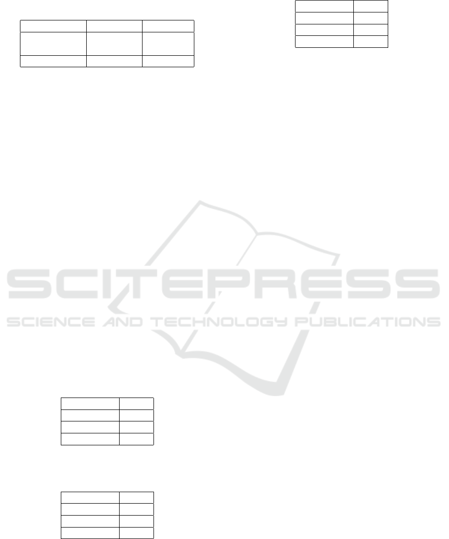
Table 2: Creating object resolution data subsets. If split

by the median of area from ground truth objects there

is an equal number of ground truth instances. However,

RPN

larger

has signiﬁcantly more background samples.

Data RPN

smaller

RPN

larger

Ground Truth 40,058 40,058

Background 3,528,370 6,370,859

Total 3,568,428 6,410,917

RPN

larger

subset, however, the skew is solely due to

the many more background examples. The ground

truth annotations are shared equally with 40,058 sam-

ples in each.

As the overall goal of object detectors is to ﬁnd

objects within the classes, the decision was made to

use the threshold of 19,205.5 to create the split in data,

despite there being signiﬁcantly more background ex-

amples in one of the datasets.

The R-FCN ensemble members were trained on

the two subsets of RPN. To evaluate how well the

expert resolution members perform on the respective

subsets of data tests were performed on splits of the

07 test data. This data was split by using the same me-

dian threshold of 19,205.5 used in creating the train-

ing subsets. Firstly, the results for small objects from

07 test can be seen in Table 3. Shown are R-FCNs

trained on RPN

smaller

, RPN

larger

and a baseline model

trained on all 07+12 data. The table shows that the

model trained towards smaller object proposals on

RPN

smaller

performs best. This trend is similarly true

for large objects as seen in Table 4. Finally, for all

ground truth objects the baseline model is the best

performing as seen in Table 5.

Table 3: Results for R-FCN models trained on three differ-

ent subsets of data and tested on only small objects from the

07 test set.

Train Data AP

RPN

smaller

55.00

RPN

larger

20.92

07+12 43.80

Table 4: Results for R-FCN models trained on three differ-

ent subsets of data and tested on only large objects from the

07 test set.

Train Data AP

RPN

smaller

21.28

RPN

larger

81.81

07+12 75.14

5.1 Image Quality Ensemble Members

To evaluate the amount of distortion in the PAS-

CAL VOC dataset a method for IQA is needed. A

Table 5: Results for R-FCN models trained on three differ-

ent subsets of data and tested on all of the 07 test set.

Train Data AP

RPN

smaller

46.74

RPN

larger

62.48

07+12 79.59

recent state of the art method is that of deep IQA

(Bosse et al., 2016). Deep IQA is a CNN-based No-

Reference (NR) IQA method that can be trained to

measure the subjective visual quality of an image.

Deep IQA consists of 14 convolutional layers, 5 max-

pooling layers and 2 fully-connected layers. The con-

volutional layers are all 3×3 convolution kernels and

activated using Rectiﬁed Linear Unit (ReLU). Inputs

to each convolutional layer are zero-padded to ensure

output size is equal to the input. Max-pooling layers

consist of 2 × 2 sized kernels. The network is trained

on mini-batches of 32 × 32 patches. During infer-

ence non-overlapping patches are sampled from the

image and image quality scores are predicted for each

instance. The patch scores are averaged for the ﬁnal

score for the entire image.

Deep IQA models were trained using the Chainer

framework (Tokui et al., 2015) as code and a model

trained for all distortions types on the LIVE dataset

were available from the deep IQA authors. How-

ever, to create a more powerful ensemble models were

ﬁne-tuned from the model provided towards each of

the 5 distortions in the LIVE. The training settings

are the same as in the deep IQA work apart from

the number of epochs in training. As ﬁne-tuning can

drastically decrease training time the epochs were de-

creased from 3,000 to 500.

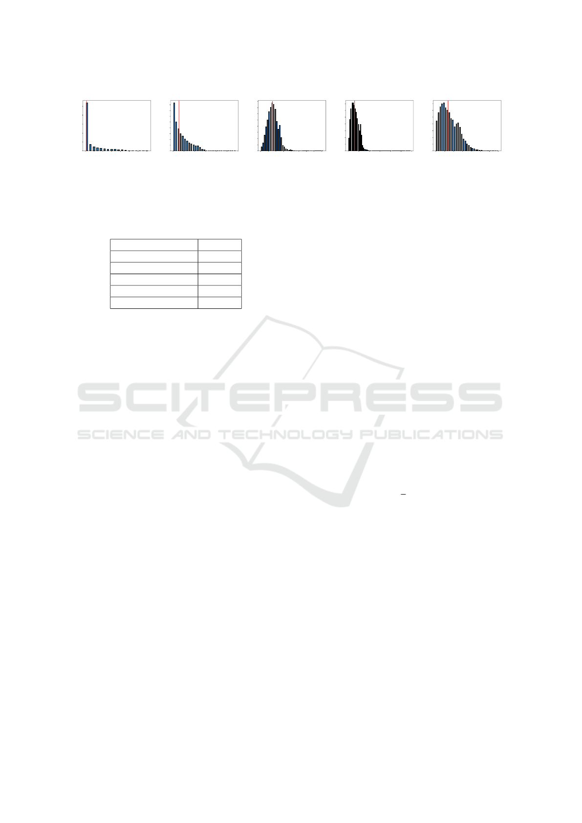
The models for each distortion type are run

through the 07+12 dataset in order to give an indica-

tion to the respective distributions. The distributions

can been seen in the histograms in Figure 3.

The distribution for white noise and Gaussian blur

is skewed towards a higher image quality and also to a

lesser extent in fast fading. Whereas the image quality

for compression distortions is somewhat of a Gaus-

sian nature. For determining an appropriate manner

to split the data the same constraints are made as in

that for object sizes, namely that both subsets of data

should have an equal number of ground truths to train

on. Again using the median for each of the ﬁve distri-

butions can satisfy this. The respective medians can

be seen in Table 6 and are shown by the red lines in

Figure 3.

It does not appear feasible to create subsets of data

for white noise image quality on 07+12. The combi-

nation of both the heavy skew and half of the data

lying below 0.599 indicates that a minimal amount

0 5 10 15 20 25 30 35

2000

4000

6000

8000

10000

Frequency

PASCAL VOC 07++12 White Noise Distribution

White Noise

0 10 20 30 40 50 60

500

1000

1500

2000

2500

3000

3500

4000

Frequency

PASCAL VOC 07++12 Gaussian Blur Distribution

Gaussian Blur

0 10 20 30 40 50 60 70 80

250

500

750

1000

1250

1500

1750

2000

Frequency

PASCAL VOC 07++12 JPEG Compression Distribution

JPEG

0 20 40 60 80 100 120

250

500

750

1000

1250

1500

1750

Frequency

PASCAL VOC 07++12 JP2K Compression Distribution

JP2K

0 10 20 30 40 50 60 70

200

400

600

800

1000

1200

1400

Frequency

PASCAL VOC 07++12 Fast Fading Distribution

Fast Fading

Figure 3: Histograms representing the distribution of image quality for the ﬁve distortions trained from the LIVE image

quality dataset. The distortions shown are white noise (a), Gaussian blur (b), JPEG compression (c), JP2k compression (d),

fast fading (e).

Table 6: Median values used for each distortion type to cre-

ate even subsets of training data from 07+12.

Distortion Type Median

White Noise 0.599

Gaussian Blur 5.607

JPEG Compression 15.660

JP2K Compression 11.747

Fast Fading 13.373

of white noise distortion is present. Therefore, this

distortion is not considered for part of the ensemble.

While the Gaussian blur image quality is also skewed

it is similar to that of the the object sizes and therefore

is deemed appropriate to split based upon its median

of 5.607. The remaining distributions are much less

skewed and a total of eight R-FCN models will be

trained for the high and low levels of image quality

for the distortions Gaussian blur, JPEG compression,

JP2K compression and fast fading. Therefore, in total

there will be ten R-FCN models trained including the

two for smaller and larger object sizes.

As in the resolution-aware R-FCN networks in-

dividual tests are run to evaluate whether or not the

models trained on the above data are candidate ex-

perts. The 07 test set is split into lower and upper

subsets for each distortion type according to their re-

spective medians. The two respective experts trained

on each of their subset and the baseline R-FCN model

are evaluated on their respective subsets. Similar re-

sults are not found in this instance as in the object

resolution experts. For each of the 5 distortions both

of the trained experts perform very similarly and are

generally 3-4 AP lower than the R-FCN model trained

on all of the data. Regardless of this result the follow-

ing section will present a method to ensemble these

members as they may still complement each other.

6 COMBINING THE ENSEMBLE

MEMBERS

The two strategies, average and weighted average, for

combining the ensemble members will be described

in this section. The method for inferring each test

image will be the same apart from the combination

step. For a given object proposal each network will

infer a bounding box and associated conﬁdence for

all classes. After this the given ensemble combina-

tion method determines the ﬁnal detection where the

conﬁdence and the four corners of the bounding box

will be averaged.

6.1 Average Ensemble

Each of the ﬁve ensemble factors are weighted evenly

in the overall ensemble. Within each ensemble factor

pair, the detection for one of the pairs will be cho-

sen and the other discarded. This is determined by

where the given factor lies for the test image in rela-

tion to the training data distribution. For example, if

it is measured that an image with a deep IQA model

to have JPEG compression below the threshold used

to split the data, then the detection found using the

model trained on that data will be used. This results

in ﬁve detections that will be weighted equally to ﬁnd

the ﬁnal detection by:

∑

i=1

i, j

(1)

where n is the number of detections found by the n en-

semble factor, p is the detection result to be averaged

and i represents one of the ensemble factors. Finally,

j is one of the ﬁve values found by each detection,

namely the four corners of the bounding-box and the

associated conﬁdence.

6.2 Weighted Average Ensemble

As in the average ensemble, each of the 10 trained

networks will be used on all object proposals found

using the RPN. Between factors, weights are dis-

tributed evenly across each of the ﬁve different types

of factors as in the average ensemble. The weighted

average ensemble is determined for each bounding

box and the associated conﬁdence by:

∑

i=1

i, j

(2)

where w

is the weight for a given detec-

tion.Weights are determined in pairs for each of the

5 ensemble factors, where the total sum of weights

is equal to n. If each detection were to be weighted

equally all w would be equal to 1. As the weights

are calculated in pairs each ensemble factor is overall

weighted equally as the pair of weights can at most

be equal to 2. By using this tactic, detections between

ensemble members can be weighted differently but

each factor is weighted equally. Weights for a given

factor are found according to where the the test image

lies for that factors training data distribution.

If the image factor result f

, for example proposal

size, is below the value used to split the data the

weights are calculated for the detection found with

the given lower network by:

Lower

= 1 +

median

− f

median

− min f

(3)

and the weight for the upper network w

U pper

by:

U pper

= 2 − w

Lower

(4)

where median

is the value used to split the train-

ing data and min f

is the minimum quality for the

given factor in the training set.

However, if the quality is above split the w

U pper

is calculated by:

U pper

= 2 −

max f

− f

max f

− median

(5)

and lower weight w

Lower

= 2 − w

U pper

. (6)

It should also be noted that outliers are not in-

cluded for the calculation of min f

and max f

by re-

moving the values below the 1% and above the 99%

percentile. This ensures that the weighing of factors

is not too heavily affected by outlier values.

7 EXPERIMENTAL RESULTS

In this section the results for the two aforementioned

ensemble combinations strategies will be presented.

When appropriate the result for the baseline R-FCN

ResNet-101 model trained on all of the 07+12 training

data and will be presented and denoted as Baseline.

The results presented will be on the 07 PASCAL VOC

test set as also shown in earlier preliminary results in

this report.

Table 7: Results for the two ensemble combination strate-

gies and for the baseline model on the 07 test set.

Method AP

Average 79.45

Weighted Average 79.47

Baseline (Dai et al., 2016) 79.59

Faster R-CNN (He et al., 2015) 76.4

YOLOv2 (Redmon and Farhadi, 2016) 78.6

The results for both combination strategies using

10 ensemble members can be seen in Table 7.

While neither of the combinations provide an im-

provement over the baseline method, both have an in-

crease in performance in comparison to their respec-

tive image quality expert results.

To the evaluate the contribution of both the eight

quality factor ensemble members and the two resolu-

tion members these were combined separately based

on the two strategies. By separating the quality and

resolution members the performance decreases by

roughly 1.0 for both in comparison the the average

ensemble result. This appears to indicate that the two

complement each other well and have their own ex-

pertise for this problem. The weighted average com-

bination strategy does not show as large of a decrease

in performance for image quality as the average com-

bination does, however, there is still a drop from 79.47

to 79.04. There is also a decrease in performance for

the two resolution members showing an AP of 77.84

on the test set. This seems to show that the addition

of weighing individual detections based on proposal

size as a poorer approach. There appears to be an in-

dication that image quality members are well suited to

adding a weight to detection. Whereas, the resolution

members are better suited to simply taking the detec-

tion from the appropriate model. The results for this

can be seen in Table 8 where both combinations are

tested. The two strategies are shown as either Image

Quality or Resolution followed by the subscript

Avg

WAvg

indicating the combination strategies of average

or weighted average respectively.

Table 8: Results for the the image quality ensemble mem-

bers and resolution members with both combinations of av-

erage and weighted average on the 07 test set.

Ensemble Members AP

Image Quality

WAvg

/ Resolution

Avg

79.83

Image Quality

Avg

/ Resolution

WAvg

79.17

Baseline (Dai et al., 2016) 79.59

Faster R-CNN (He et al., 2015) 76.4

YOLOv2 (Redmon and Farhadi, 2016) 78.6

Results in Table 8 show that by using separate

strategies where image quality members are weighted

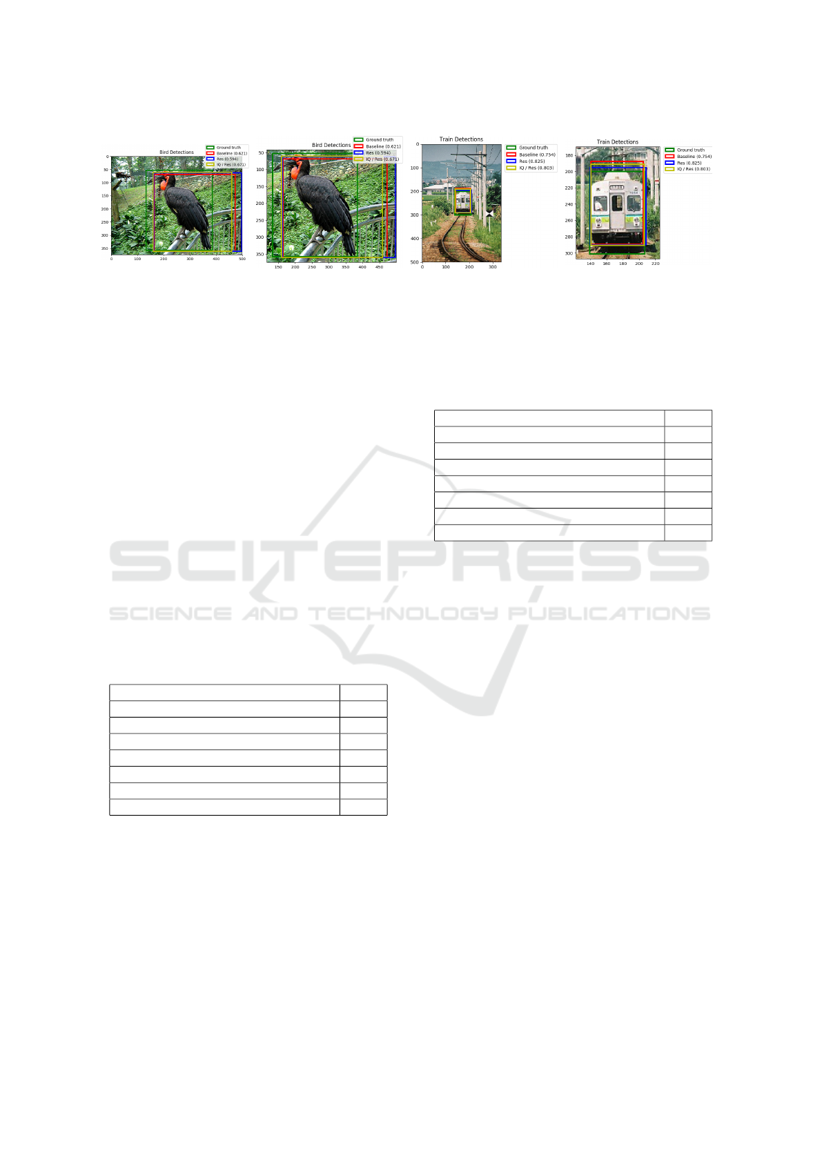
Figure 4: Detections for the bird class from an image in the 07 test set. Shown are the bounding boxes for the ground truth

annotation, baseline, Resolution

base

(Res) and Image Quality

WAvg

/ Resolution

Avgbase

(IQ / Res). The Intersection-Over-Union

(IoU) between the ground truth and bounding box is shown in parentheses for each method.

and when resolution members are averaged only in-

creases the performance. Additionally, the perfor-

mance surpasses the baseline model.

The results so far have only been with different

combinations of the expert ensemble members. An-

other strategy is to include the baseline model trained

on all of the 07+12 data. As the baseline model per-

forms well by itself the other ensemble members will

act as support It should be noted that as there is no

complementary member to the baseline. Therefore,

its detections are weighted by 1.0 regardless of en-

semble combination strategy. Firstly, the results for

the average and weighted average ensemble can be

seen in Table 9. The inclusion of the baseline model is

shown by the subscript

base

. Performance is increased

in both cases, the weighted average is increased by

0.22. While the average strategy is increased by 0.43.

Table 9: Results for the two ensemble combination strate-

gies and for the baseline model on the 07 test set. Shown

is both the results with the expert ensemble members only

and experts plus the baseline model.

Method AP

Average 79.45

Average

base

79.88

Weighted Average 79.47

Weighted Average

base

79.69

Baseline (Dai et al., 2016) 79.59

Faster R-CNN (He et al., 2015) 76.4

YOLOv2 (Redmon and Farhadi, 2016) 78.6

The addition of the baseline model to the ensem-

ble using different strategies for the two factors can

be seen in Table 10. This provided the best result of

any ensemble combination. Image quality with the

weighted average and resolution with average ensem-

ble results in 80.09, an increase of 0.50 in comparison

to the baseline R-FCN.

The AP results for each category for the Image

Quality

WAvg

/ Resolution

Avgbase

ensemble can be seen

in Table 11. The tables show results for the baseline

model, the given ensemble method and the difference

Table 10: Results for the the image quality ensemble mem-

bers and resolution members with both combinations of av-

erage and weighted average on the 07 test set. Shown is

both the results with the expert ensemble members only and

experts plus the baseline model.

Ensemble Members AP

Image Quality

WAvg

/ Resolution

Avg

79.83

Image Quality

WAvg

/ Resolution

Avg

base

80.09

Image Quality

Avg

/ Resolution

WAvg

79.17

Image Quality

Avg

/ Resolution

WAvg

base

79.54

Baseline (Dai et al., 2016) 79.59

Faster R-CNN (He et al., 2015) 76.4

YOLOv2 (Redmon and Farhadi, 2016) 78.6

between the two for a given class.

Finally, two examples of detections can be seen in

Figure 4. For both instances, on the left is the full size

image and right a zoomed version of the object and

detections. The detections shown are for the ground

truth annotation, baseline, Resolution

base

(Res) and

Image Quality

WAvg

/ Resolution

Avgbase

(IQ / Res). Ad-

ditionally, shown in parentheses in the legend is the

IoU between the ground truth and detection for the

given method.

8 CONCLUSION AND FUTURE

WORK

This work has presented a method for creating an en-

semble of R-FCNs trained towards object resolution

and image quality using the PASCAL VOC dataset. If

combined appropriately an improvement against the

standard R-FCN method can be obtained. Address-

ing items such as the skew in factor distributions data

may help create better individual members and create

a stronger ensemble.

This work uses R-FCN as the backbones, how-

ever, any object detection method could be used and

shows the possibilities of engineering towards spe-

ciﬁc challenges in object detection.

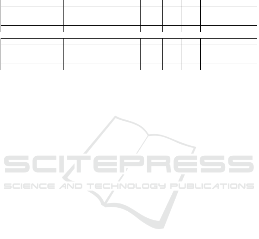
Table 11: Results for the individual classes in the 07 test set. Shown are the results for the baseline model and Image

Quality

WAvg

/ Resolution

Avgbase

. Additionally the difference between the two methods are presented for a given class.

Model aero bike bird boat bottle bus car cat chair cow

Baseline (Dai et al., 2016) 80.53 84.59 79.89 71.52 67.54 87.22 87.59 87.98 65.15 87.11

Image Quality

WAvg

Resolution

Avgbase

80.57 85.45 81.02 72.51 68.69 88.00 87.38 89.13 67.27 86.57

Difference +0.04 +0.86 +1.13 +0.99 +1.15 +0.78 -0.21 +1.15 +2.12 -0.54

Model table dog horse mbike person plant sheep sofa train tv

Baseline (Dai et al., 2016) 73.66 88.61 87.83 83.21 79.87 54.60 84.07 80.03 83.60 77.17

Image Quality

WAvg

Resolution

Avgbase

72.21 88.75 87.04 84.15 80.17 53.97 83.56 80.11 86.62 78.64

Difference -1.45 +0.14 -0.79 +0.95 +0.30 -0.63 -0.51 +0.08 +3.02 +1.47

REFERENCES

Bosse, S., Maniry, D., M

uller, K., Wiegand, T., and Samek,

W. (2016). Deep neural networks for no-reference

and full-reference image quality assessment. CoRR,

abs/1612.01697.

COCO, M. (2017). Ms coco detections leaderboard.

Dai, J., Li, Y., He, K., and Sun, J. (2016). R-FCN: object de-

tection via region-based fully convolutional networks.

CoRR, abs/1605.06409.

Everingham, M., Van Gool, L., Williams, C. K. I., Winn,

J., and Zisserman, A. (2010). The pascal visual ob-

ject classes (voc) challenge. International Journal of

Computer Vision, 88(2):303–338.

Girshick, R. (2015). Fast R-CNN. In Proceedings of the

International Conference on Computer Vision (ICCV).

Girshick, R., Donahue, J., Darrell, T., and Malik, J. (2014).

Rich feature hierarchies for accurate object detec-

tion and semantic segmentation. In Proceedings of

the IEEE conference on computer vision and pattern

recognition, pages 580–587.

He, K., Zhang, X., Ren, S., and Sun, J. (2015). Deep

residual learning for image recognition. CoRR,

abs/1512.03385.

Huang, J., Rathod, V., Sun, C., Zhu, M., Korattikara, A.,

Fathi, A., Fischer, I., Wojna, Z., Song, Y., Guadar-

rama, S., and Murphy, K. (2016). Speed/accuracy

trade-offs for modern convolutional object detectors.

CoRR, abs/1611.10012.

Jia, Y., Shelhamer, E., Donahue, J., Karayev, S., Long, J.,

Girshick, R., Guadarrama, S., and Darrell, T. (2014).

Caffe: Convolutional architecture for fast feature em-

bedding. arXiv preprint arXiv:1408.5093.

Krizhevsky, A., Sutskever, I., and Hinton, G. E. (2012).

Imagenet classiﬁcation with deep convolutional neu-

ral networks. In Pereira, F., Burges, C. J. C., Bottou,

L., and Weinberger, K. Q., editors, Advances in Neu-

ral Information Processing Systems 25, pages 1097–

1105. Curran Associates, Inc.

Larson, E. and Chandler, D. M. (2009). Consumer subjec-

tive image quality database.

Li, Y., Qi, H., Dai, J., Ji, X., and Wei, Y. (2016). Fully

convolutional instance-aware semantic segmentation.

CoRR, abs/1611.07709.

Lin, T.-Y., Maire, M., Belongie, S., Hays, J., Perona, P.,

Ramanan, D., Doll

ar, P., and Zitnick, C. L. (2014).

Microsoft COCO: Common Objects in Context, pages

740–755. Springer International Publishing, Cham.

Ponomarenko, N., Ieremeiev, O., Lukin, V., Egiazarian, K.,

Jin, L., Astola, J., Vozel, B., Chehdi, K., Carli, M.,

Battisti, F., and Kuo, C. C. J. (2013). Color image

database tid2013: Peculiarities and preliminary re-

sults. In European Workshop on Visual Information

Processing (EUVIP), pages 106–111.

Redmon, J. and Farhadi, A. (2016). YOLO9000: better,

faster, stronger. CoRR, abs/1612.08242.

Ren, S., He, K., Girshick, R., and Sun, J. (2015). Faster R-

CNN: Towards real-time object detection with region

proposal networks. In Neural Information Processing

Systems (NIPS).

Russakovsky, O., Deng, J., Su, H., Krause, J., Satheesh,

S., Ma, S., Huang, Z., Karpathy, A., Khosla, A.,

Bernstein, M., Berg, A. C., and Fei-Fei, L. (2015).

ImageNet Large Scale Visual Recognition Challenge.

International Journal of Computer Vision (IJCV),

115(3):211–252.

Schroff, F. (2009). Semantic Image Segmentation and Web-

supervised Visual Learning. University of Oxford.

Sheikh, H. R., Sabir, M. F., and Bovik, A. C. Live image

quality assessment database release 2.

Sheikh, H. R., Sabir, M. F., and Bovik, A. C. (2006). A sta-

tistical evaluation of recent full reference image qual-

ity assessment algorithms. IEEE Transactions on Im-

age Processing, 15(11):3440–3451.

Shrivastava, A., Gupta, A., and Girshick, R. B. (2016).

Training region-based object detectors with online

hard example mining. CoRR, abs/1604.03540.

Simonyan, K. and Zisserman, A. (2015). Very deep convo-

lutional networks for large-scale image recognition. In

ICLR.

Szegedy, C., Ioffe, S., and Vanhoucke, V. (2016). Inception-

v4, inception-resnet and the impact of residual con-

nections on learning. CoRR, abs/1602.07261.

Tokui, S., Oono, K., Hido, S., and Clayton, J. (2015).

Chainer: a next-generation open source framework for

deep learning. In Proceedings of Workshop on Ma-

chine Learning Systems (LearningSys) in The Twenty-

ninth Annual Conference on Neural Information Pro-

cessing Systems (NIPS).

Uijlings, J. R. R., van de Sande, K. E. A., Gevers, T., and

Smeulders, A. W. M. (2013). Selective search for ob-

ject recognition. International Journal of Computer

Vision, 104(2):154–171.

Zhang, C. and Ma, Y. (2012). Ensemble Machine Learning.

Springer US.

Zhang, X., Yang, Y.-H., Han, Z., Wang, H., and Gao, C.

(2013). Object class detection: A survey. ACM Com-

put. Surv., 46(1):10:1–10:53.