
Depth Value Pre-Processing for Accurate Transfer Learning based
RGB-D Object Recognition
Andreas Aakerberg, Kamal Nasrollahi, Christoffer B. Rasmussen and Thomas B. Moeslund
Aalborg University, Rendsburggade 14, 9000 Aalborg, Denmark
Keywords:
Deep Learning, Computer Vision, Artificial Vision, RGB-D, Convolutional Neural Networks, Transfer
Learning, Surface Normals.
Abstract:
Object recognition is one of the important tasks in computer vision which has found enormous applications.
Depth modality is proven to provide supplementary information to the common RGB modality for object
recognition. In this paper, we propose methods to improve the recognition performance of an existing deep
learning based RGB-D object recognition model, namely the FusionNet proposed by Eitel et al. First, we show
that encoding the depth values as colorized surface normals is beneficial, when the model is initialized with
weights learned from training on ImageNet data. Additionally, we show that the RGB stream of the FusionNet
model can benefit from using deeper network architectures, namely the 16-layered VGGNet, in exchange for
the 8-layered CaffeNet. In combination, these changes improves the recognition performance with 2.2% in
comparison to the original FusionNet, when evaluating on the Washington RGB-D Object Dataset.
1 INTRODUCTION
Computer vision is one of the most import sensor
technologies for a number of industrial applications,
and for facilitating tomorrows intelligent assistant
systems. The field of computer vision includes meth-
ods for acquiring, processing, analyzing and under-
standing images in order to make automated actions
and intelligent decisions. This is highly useful in a
number of applications such as surveillance drones,
quality inspection in assembly lines and self-driving
cars.
In this paper, we address the problem of ob-
ject recognition, a field within artificial intelligence,
which deals with making a machine capable of iden-
tifying the type of object depicted in an image. While
successful RGB based object recognition models al-
ready exists, recent advancements within range imag-
ing technologies has made researchers experiment
with using RGB-Depth (RGB-D) data to further in-
crease the recognition performance. This is possi-
ble, as the depth data contains additional geometric
information about the object shapes, besides the tex-
ture, color and appearance information already con-
tained in the Red Green and Blue (RGB) data. The
depth data is furthermore invariant to lighting and
color variations, allowing for a potentially more ro-
bust classifier (Guo et al., 2014). A recent example
of using both the RGB and depth modality for object
recognition is the FusionNet model proposed by (Ei-
tel et al., 2015). This model is based on two Convolu-
tional Neural Network (CNN) streams, pre-trained on
ImageNet data (Russakovsky et al., 2015), which op-
erates separately on RGB and depth data. Using a late
fusion approach, a higher level abstraction from the
features extracted by the two CNNs are created to en-
able multi-modal object recognition with high accu-
racy. The two streams are based on the CaffeNet, and
pre-processing of the depth values is performed by
color encoding the depth values with a Jet colormap,
for efficient use of the models pre-trained on natural
images. However, we argue that this pre-processing
method is sub-optimal, as it results in images with lit-
tle structural information. Additionally, we argue that
the model capacity of the CaffeNet is too low for opti-
mal learning from the dataset. To this end we propose
a novel depth value pre-processing method based on
colorized surface normals, and show that for the RGB
stream, the deeper VGGNet (Simonyan and Zisser-
man, 2014) is superior over the CaffeNet, when eval-
uating on the Washington RGB-D object dataset (Lai
et al., 2011).
Aakerberg A., Nasrollahi K., Rasmussen C. and Moeslund T.
Depth Value Pre-Processing for Accurate Transfer Learning based RGB-D Object Recognition.
DOI: 10.5220/0006511501210128
In Proceedings of the 9th International Joint Conference on Computational Intelligence (IJCCI 2017), pages 121-128
ISBN: 978-989-758-274-5
Copyright
c
2017 by SCITEPRESS – Science and Technology Publications, Lda. All rights reserved
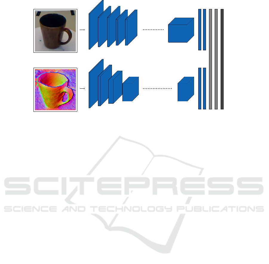
RGB image
Depth image
input
conv
conv
conv conv
input
conv conv
conv conv
conv
fc
fc
fc
fc fus fus
softmax
Figure 1: Simplified overview of the architecture of the proposed deep learning based object recognition model.
2 RELATED WORK
Our work is related to several research fields, includ-
ing CNNs for object recognition and object recog-
nition from RGB-D data. This section highlights
the most relevant related work to our approach. Al-
though many successful classical computer vision al-
gorithms, based on feature descriptors such as Scale
Invariant Feature Transform (SIFT) (Lowe, 2004) and
Speeded Up Robust Features (SURF) (Bay et al.,
2008), exists for image classification, recent advance-
ments within deep learning have made the classical
methods inferior in comparison, for a wide range of
applications. This was widely recognized in 2012
when Krizhevsky et al. won the prestigious Im-
ageNet Large-Scale Visual Recognition Challenge
(ILSVRC) (Russakovsky et al., 2015) using a deep
CNN (Krizhevsky et al., 2012) to achieve 10.9% bet-
ter classification accuracy, compared to the second
best entry based on a classical method. Deep learning
based models for image classification has continued
to evolve into deeper and more complex models such
as the 16-layered VGGNet (Simonyan and Zisserman,
2014), the GoogleNet based on several Inception
Modules allowing for parallel sections in the network
(Szegedy et al., 2014), and the very deep 152-layered
ResNet (He et al., 2015) facilitating residual learning.
One of the first uses CNNs for RGB-D object recogni-
tion was proposed by (Socher et al., 2012), and relied
on a combination of CNNs for feature extraction and
Recursive Neural Networks (RNNs) for creation of
higher level abstractions and classification. However,
work by (Yosinski et al., 2014) and (Razavian et al.,
2014) among others, has shown that features extracted
from CNNs are reusable for novel generic tasks, in-
dicating that deep architectures can be fine-tuned to
related problems, even when very little new training
data is available. This was used by (Eitel et al., 2015),
which proposed a multi-modal RGB-D object recog-
nition model based on two CNN pre-trained on Ima-
geNet data, and fine-tuned to the Washington RGB-
D object dataset. To efficiently use the filters previ-
ously learned in the CNNs, different encoding meth-
ods of the depth values was evaluated. The authors
found that a Jet color encoding of the depth values
resulted in the best recognition performance. Other
approaches to efficient learning from the depth data
includes (Li et al., 2015), where dense local features
were extracted from the depth data and encoded as
Fisher vectors, instead of using a colorization method.
In (Carlucci et al., 2016) a large database, with more
than 4 million synthesized depth images, was created
for the purpose of training a CNN on raw depth data.
In (Wang et al., 2016) features from both the RGB
and depth data is learned jointly, to exploit both share-
able and modality-specific information. Encoding of
the depth values was done by computing the surface
normal for each pixel. A multi-modal object recogni-
tion model, where the depth network is pre-trained on
Computer-aided design (CAD) data to eliminate the
need for color mapping of the depth data is proposed
in (Sun et al., 2017). In (Asif et al., 2017), hierarchi-
cal cascaded forests were used for computing grasp-
poses and perform object recognition, using a num-
ber of different features, including surface normals,
jet colorized depth values, and orientation angle maps
to capture object appearance and structure.
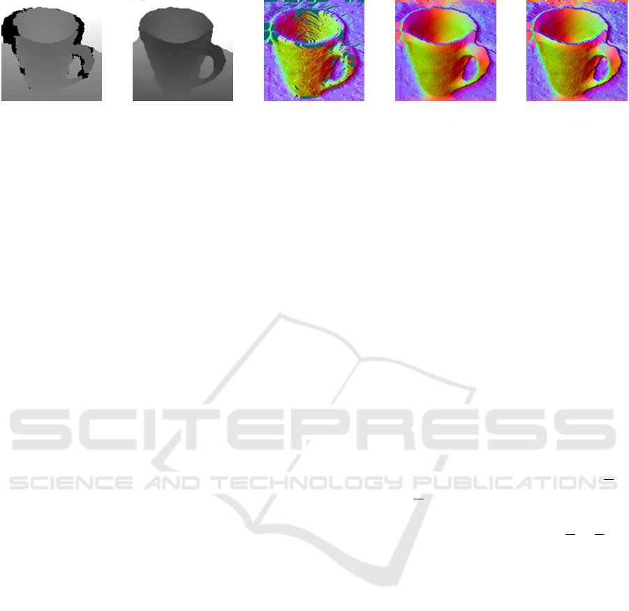
(a) (b) (c) (d) (e)
Figure 2: Visualization of the steps in the proposed depth image pre-processing method. (a) Raw depth image (converted
to greyscale for visualization purposes), (b) After reconstruction of missing depth values, (c) Colorized surface normals
without prior depth value smoothing, (d) Colorized surface normals with prior bilateral smoothing of depth values, (e) After
sharpening.
3 PROPOSED APPROACH
Our approach adopts the FusionNet concept proposed
by (Eitel et al., 2015). Hence we develop a multi-
modal RGB-D object recognition model consisting of
two CNNs streams, pre-trained on ImageNet data, op-
erating on RGB and depth data respectively. A late
fusion approach is used to combine features extracted
by the two streams, effectively creating a multi-modal
classifier which creates higher level representations of
features from the two modalities. Different from (Ei-
tel et al., 2015) we use a deeper network architecture
for the RGB stream, and rely on colorized surface nor-
mals for encoding of the depth values.
3.1 RGB-D Image Pre-Processing
Both the RGB and depth data needs to be pre-
processed before it can be used in combination with
CNNs pre-trained on ImageNet data. As in (Eitel
et al., 2015) we square images from both domains us-
ing border replication of pixels on the longer sides,
and re-size them to 256 × 256 pixels. During train-
ing and inference the images are either randomly
cropped, or center cropped to match the input dimen-
sions of the respective CNNs. While the RGB images
need no further processing, the depth images have to
be transferred to the RGB domain to benefit from the
features learned in the CNNs pre-trained on natural
images. The proposed pre-processing method for the
depth values is based on a number of key observa-
tions. First of, in depth images strong discontinuities
are in fact edges, and not just texture or color transi-
tions, like it could be the case in RGB images, and
these can be useful features to extract. Secondly, the
outline of an object can be helpful to identify the re-
spective class of an object, when no true object color
information is present. Lastly, curvature information
is more present in depth images than RGB images.
To enable the creation of colorized surface normal
images with homogeneous surface areas, we start by
reconstructing the missing depth values in the depth
images, using the recursive median filter proposed in
(Lai et al., 2011). Hence we recursively apply a me-
dian filter which only considers non-missing values
in small neighbourhood around a pixel with missing
depth values. This minimizes blurring of the depth
images and effectively fill all missing depth values.
We use a kernel size is of 5 × 5, and use padding
with border replication to solve the border problem
when applying the filter. As the depth images also
contain noise, we subsequently filter the depth im-
ages using a bilateral filter. This filter provides a good
compromise, between preserving edges and sufficient
smoothing, for this application. Next, we compute
the surface normals for each pixel in the depth im-
age. We define two orthogonal tangent vectors, par-
allel to the x and y-axis are defined as x = [1,0,
∂z
∂x
]
T
and y = [0,1,
∂z
∂y
]
T
. As the surface normal n is de-
fined as the cross-product between x and y the sur-
face normal n can be expressed as n = (−
∂z
∂x
,−
∂z
∂y
,1).
The resulting surface normal n is then normalized to
a unit vector using the Euclidean norm. As the x,y,z
values of the normalized surface normal n = [x, y, z]
T
lie in the range [−1, 1] these are mapped to integer
values ∈ [0,255] before being assigned as RGB val-
ues where R ← x,G ← y,B ← z. Even though the
bilateral filter used to smooth the depth values, aims
to preserve edges, some details are lost in the pro-
cess. While these can’t be recovered without the use
of more involved methods such as super-resolution,
the image can still be sharpened to enhance the ap-
pearance of edges and fine-details, which can help the
CNN learn relevant features from the image. Hence
the image is sharpened using the unsharp mask fil-
ter, which increases contrast around edges and other
high-frequency components. An example of the re-
sulting depth image after each step in the proposed
pre-processing method can be seen in Figure 2. By
visual inspection, we find the use of colorized sur-
face normals better captures structural information,
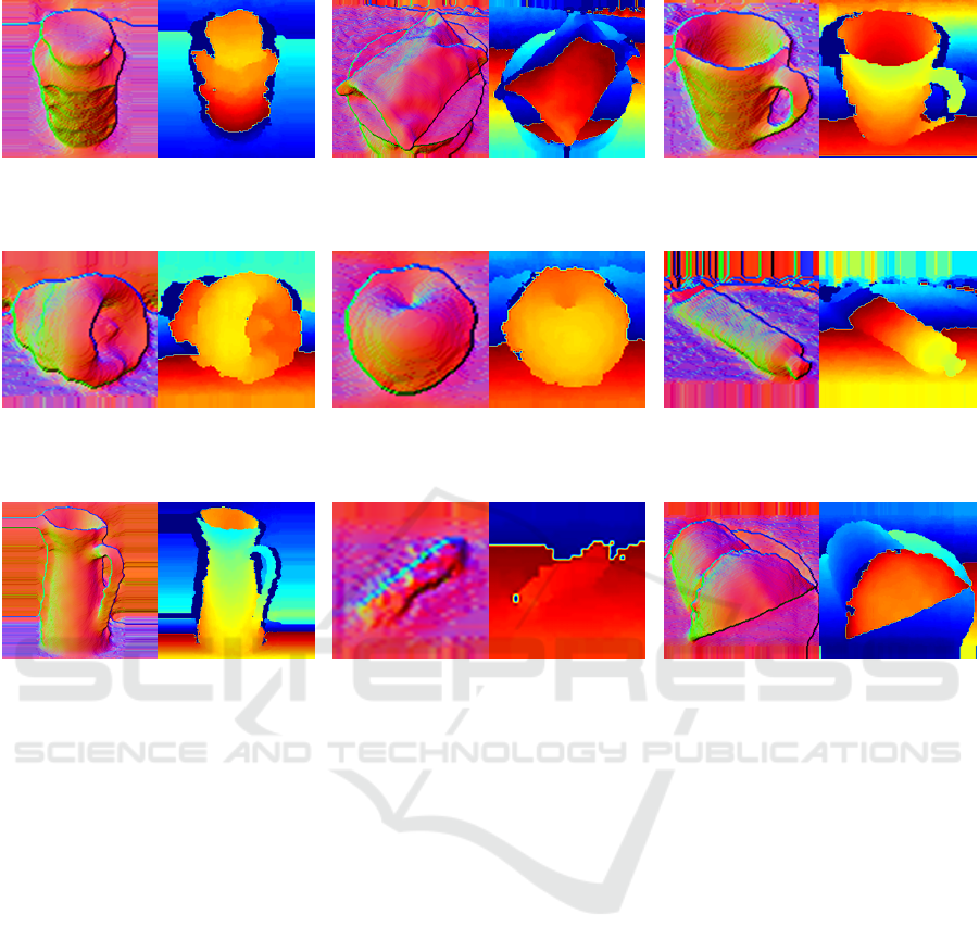
(a) (b) (a) (b) (a) (b)
Figure 3: Visualization of pre-processing methods. (a) This work, (b) (Eitel et al., 2015). The visualized objects are, from left
to right: ’Food Jar’, ’Food Bag’ and ’Coffee Mug’.
(a) (b) (a) (b) (a) (b)
Figure 4: Visualization of pre-processing methods. (a) This work, (b) (Eitel et al., 2015). The visualized objects are, from left
to right: ’Bell Pepper’, ’Pear’ and ’Toothpaste’.
(a) (b) (a) (b) (a) (b)
Figure 5: Visualization of pre-processing methods. (a) This work, (b) (Eitel et al., 2015). The visualized objects are, from left
to right: ’Pitcher’, ’Dry Battery’ and ’Cap’.
and fine details of the objects, than the Jet coloriza-
tion method. The surface normal encoding method is
furthermore independent of the distance to the camera
and the total depth space covered in the depth images.
A comparison of our pre-processing method to the Jet
colorization method can be seen in Figure 3, Figure 4
and Figure 5.
3.2 Model Architecture
Similar to (Eitel et al., 2015), we use the CaffeNet
for the depth stream. This network is a variant of
the AlexNet (Krizhevsky et al., 2012), consisting of
5 convolutional layers and 3 fully connected layers.
In a preliminary experiment, using the 16-layered
VGGNet, consisting of 13 convolutional layers and
3 fully connected layers, for the depth stream did
not show any improvement of the recognition perfor-
mance. On the contrary, the use of the 16-layered VG-
GNet was found to significantly improve the recog-
nition performance of the RGB stream. Hence the
CaffeNet and the VGGNet are used to extract fea-
tures from the pre-processed RGB and depth images
respectively. Following the FusionNet concept, we
remove the softmax layers, and concatenate the fc-
7 layer responses of each stream, and use these as
input to a fully connected fusion layer followed by
a softmax classification layer, performing classifica-
tion with respect to the 51-classes in the Washington
RGB-D object dataset. The resulting network archi-
tecture can be seen in Figure 1.
3.3 Network Training
We initialize both streams with the weights values ob-
tained by pre-training on ImageNet data. We then
proceed with fine-tuning each stream separately to
the Washington RGB-D object dataset. For the depth
stream, we used two training steps. First, we fine-
tuned all layers for 30,000 iterations using a base
learning rate of 0.01, which was dropped to 0.001 af-
ter 20,000 iterations. A momentum of 0.9, a weight
decay of 0.0002, a batch size of 128 and the SGD
solver was used. Next, we continue fine-tuning only
the fully connected layers, using a base learning rate
of 0.01 which is dropped to 0.005 and 0.0025 at 2000
and 4000 iterations respectively. To control overfit-
ting the weight decay is doubled to 0.0004, and the
mushroom
peach
pitcher
camera
pear
ball
potato
coffeemug
lightbulb
rubbereraser
bowl
bellpepper
calculator
foodjar
shampoo
apple
garlic
stapler
foodbox
plate
cap
sodacan
tomato
onion
cellphone
foodbag
kleenex
waterbottle
drybattery
keyboard
comb
toothbrush
flashlight
sponge
binder
foodcan
foodcup
lemon
lime
orange
scissors
toothpaste
banana
cerealbox
gluestick
greens
handtowel
instantnoodles
marker
notebook
pliers
0.2
0.4
0.6
0.8
1
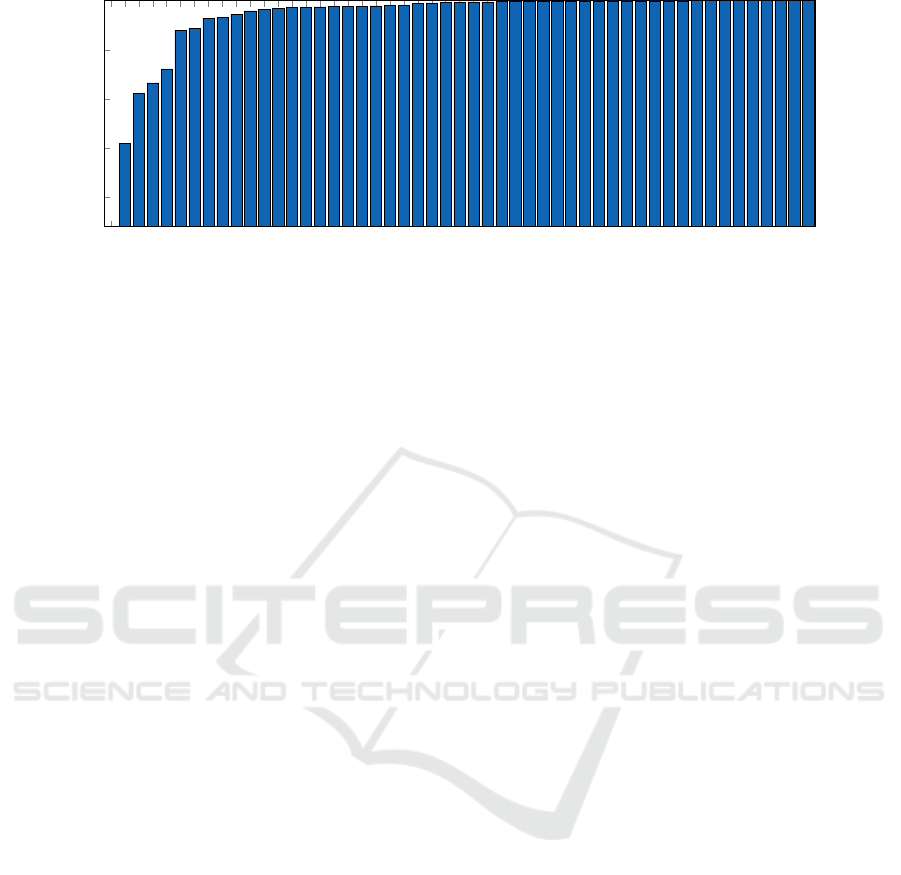
Figure 6: The per-class recall of the proposed model, averaged over all ten splits.
momentum is increased to 0.95 and the batch size
is increased to 256. For the RGB stream, we fine-
tuned all fully connected layers only, for 12,000 it-
erations using a base learning rate of 0.001 which
was dropped to 0.0001 and 0.00001 after 5000 and
10,000 iterations respectively. A momentum of 0.9,
a weight decay of 0.0005, a batch size of 80, ob-
tained using 2× gradient accumulation, and the SGD
solver was used. The fusion net was trained by freez-
ing the weights in the individual streams, and only
learning the weights in the fully connected layers
of the fusion network. We trained the fusion net-
work for 3,000 iterations, with a base learning rate
of 0.02 which followed a polynomial decay defined
as BaseLR · (1 − Iteration/Maxiteration)
0.5
. A mo-
mentum of 0.9, a weight decay of 0.0005, a batch size
of 80, obtained using 2× gradient accumulation, and
the SGD solver was used. The number of training
iterations and hyper-parameters was found based on
the performance on a validation set in a preliminary
experiment.
4 EXPERIMENTAL RESULTS
We perform all our experiments using the Caffe deep
learning framework (Jia et al., 2014), and use random
cropping and horizontal flipping of the training im-
ages for data augmentation. During training and in-
ference, we subtract the mean RGB and depth image
from the input images, to center the data.
4.1 RGB-D Object Dataset
We use the Washington RGB-D object dataset (Lai
et al., 2011) for training and evaluation of the pro-
posed models. This dataset contains 207,920 RGB-D
images of common household objects, all captured in
a controlled environment using a spinning table and a
Prime-Sense prototype RGB-D camera, similar to the
Microsoft Kinect V1 camera. The RGB and depth in-
formation are stored in separate files, where the depth
images files contain the depth in millimeters, stored
in a single-channel image in the uint16 format, and
the RGB information is stored in three-channel uint8
RGB images. The images are recorded continuously
at 20 Hz, and organized into 51 classes, which con-
tains images of three to 10 different instances of ob-
jects of the same class, making a total of 300 distinct
objects. There are several hundred images of each
instance captured under three different viewpoint an-
gles, namely 30
◦
, 45
◦
. and 60
◦
. In combination with
the dataset, the authors also present a method for sub-
sampling the dataset, and 10 pre-defined training and
test splits for cross-validation, which is adopted in this
work, and nearly all State-of-the-Art (SoTA) works
using this dataset. The dataset is subsampled by tak-
ing every fifth frame, resulting in 41,877 RGB-D im-
ages for training and evaluation. For each split, one
random object instance from each class is left out
from the training set and used for testing. Training
is performed on images of the remaining (300 − 51)
249 instances. This results in roughly 35,000 training
images and 7,000 testing images in each split. At test
time, the classifier has to assign the correct label to a
previously unseen object instance from each of the 51
classes.
4.2 Recognition Performance
When evaluated on all ten splits from the Washing-
ton RGB-D object dataset, the average performance
of the individual streams was found to be 89.5 ±1.0
and 84.5 ±2.9 for the RGB and depth streams re-
spectively. Hence, the use of the 16-layered VGGNet
for the RGB-stream results in 5.4% higher recogni-
pitcher
camera
peach
binder
mushroom
comb
scissors
lightbulb
lime
cap
cellphone
banana
orange
greens
keyboard
cerealbox
calculator
flashlight
toothbrush
rubbereraser
apple
drybattery
pliers
sodacan
potato
lemon
bowl
bellpepper
kleenex
handtowel
notebook
foodcup
toothpaste
pear
plate
gluestick
onion
foodjar
shampoo
coffeemug
stapler
tomato
garlic
ball
waterbottle
foodbag
instantnoodles
marker
sponge
foodbox
foodcan
400
600
800
1,000
1,200
1,400
1,600
1,800
2,000
2,200
Number of RGB-D images
Figure 7: Visualization of the class imbalance of all ten splits in Washington RGB-D object dataset. Red bars indicate the
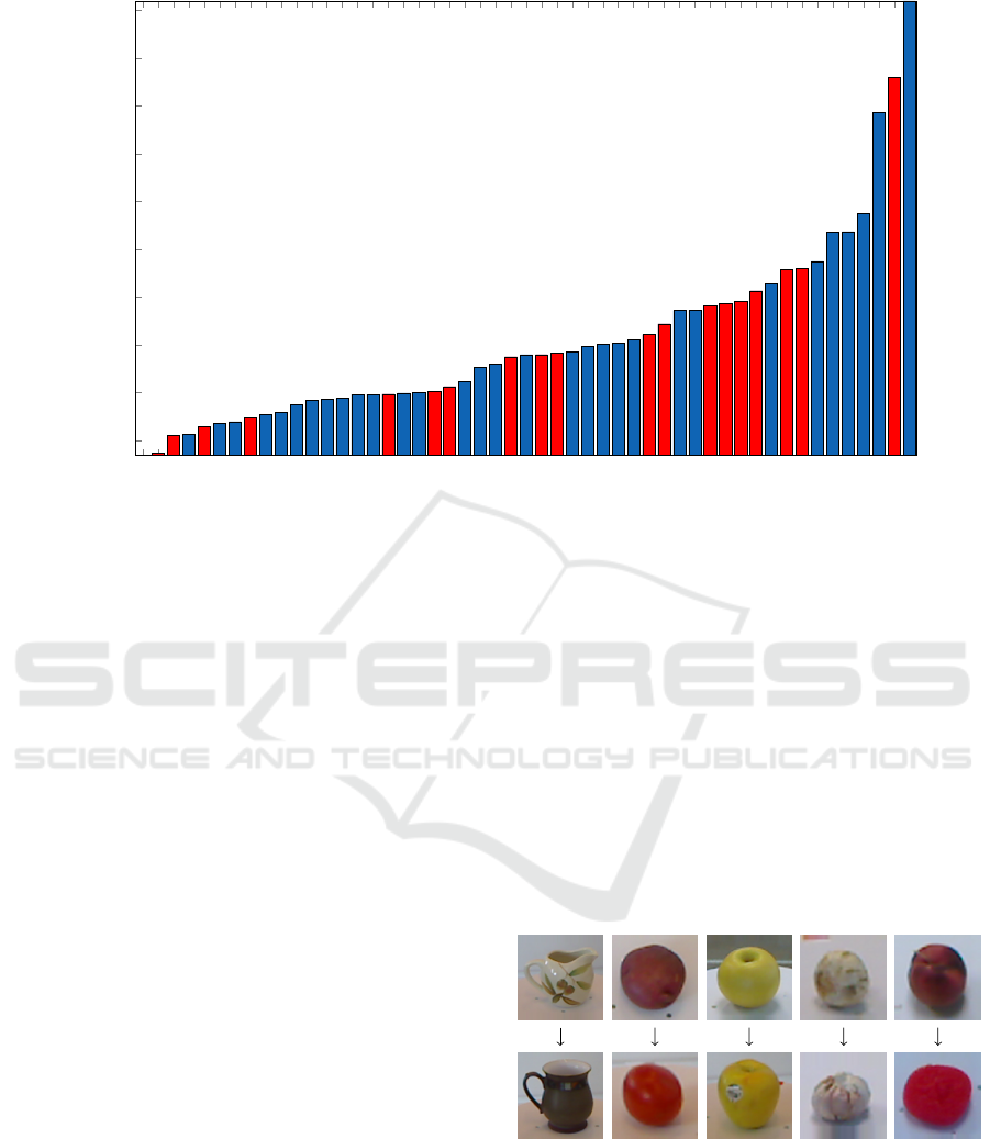
20-classes on which the proposed model has a recall lower than 0.98% averaged on all ten splits.
tion accuracy in comparison to the 8-layered Caf-
feNet used in the original FusionNet. Reconstruct-
ing the missing depth values, filtering and encoding
them as colorized surface normals results in 0.7%
higher recognition accuracy on average, compared to
colorizing the depth values using the Jet encoding
method. In combination these changes resulted in an
average accuracy of 93.5 ± 1.1% for the proposed
model, which is 2.2% higher than the original Fusion-
Net.
As seen in Figure 6, the proposed model has a re-
call that is >98% on 31 out of the 51 classes in the
dataset. By inspecting images of class instances in the
dataset, it was found that some instances are in fact
easily confused with each other. This is illustrated in
Figure 8, which shows examples of typical misclassi-
fications made by the proposed model. In these par-
itcular cases, the depth data provides little extra infor-
mation which can be used to distinguish between the
object classes.
5 DISCUSSION
While the use of a deeper network architecture for the
RGB stream in the FusionNet resulted in improved
recognition performance, this was however not the
case for the depth stream. Hence the performance of
this stream is hypothesized to be bound by the dataset,
and not model capacity. In addition to large areas with
missing depth values in the depth images, analysis of
the dataset has shown that this is imbalanced in an
unfavorable way to some objects with a low recall, as
visualized in Figure 7. One could possibly address
the this, by balancing the dataset. Furthermore, it was
found that some classes in the dataset consists of only
three unique object instances, while others contains
to 10. This might also limit how well a trained model
will be able to generalize to unseen examples.
(a) (b) (c) (d) (e)
Figure 8: Examples of typical misclassifications. The first
row shows images of the actual class. (a) ’Pitcher’→ ’Coffe
mug’, (b) ’Potato’→ ’Tomato’, (c) ’Pear’→ ’Apple’, (d)
’Mushroom’→ ’Garlic’, (e) ’Peach’→ ’Sponge’.
Table 1: Comparison of the models proposed in this work to SoTA works. Red and blue indicates best and second best
performance respectively.
Method RGB Depth RGB-D
Nonlinear SVM (Lai et al., 2011) 74.5 ± 3.1 64.7 ± 2.2 83.9 ± 3.5
CNN-RNN (Socher et al., 2012) 80.8 ± 4.2 78.9 ± 3.8 86.8 ± 3.3
FusionNet (Eitel et al., 2015) 84.1 ± 2.7 83.8 ± 2.7 91.3 ± 1.4
CNN+Fisher (Li et al., 2015) 90.8 ± 1.6 81.8 ± 2.4 93.8 ± 0.9
DepthNet (Carlucci et al., 2016) 88.4 ± 1.8 83.8 ± 2.0 92.2 ± 1.3
1
CIMDL (Wang et al., 2016) 87.3 ± 1.6 84.2 ± 1.7 92.4 ± 1.8
DCNN-GPC (Sun et al., 2017) 88.4 ± 2.1 80.3 ± 2.7 91.8 ± 1.1
STEM-CaRFs (Asif et al., 2017) 88.8 ± 2.0 80.8 ± 2.1 92.2 ± 1.3
This work 89.5 ± 1.9 84.5 ± 2.9 93.5 ± 1.1
6 CONCLUSION
The FusionNet model for object recognition proposed
by (Eitel et al., 2015), showed promising results with
the use of a two streamed CNNs architecture, based
on the 8-layered CaffeNet, and a simple Jet color map
based encoding method for the depth values. In this
work, we have shown that the FusionNet model can
be improved by encoding the depth values as col-
orized surface normals, and by using the deeper 16-
layered VGGNet for the RGB stream. The improve-
ment in recognition performance is mainly due to the
larger capacity of the VGGNet, but also due to depth
values encoded as colorized surface normals, better
captures structural and curvature information of ob-
jects. When evaluating on the Washington RGB-D
object dataset, these changes was found to result in
an accuracy of 93.5%, which is 2.2% higher than the
original FusionNet proposed by (Eitel et al., 2015),
and competitive with current SoTA works.
REFERENCES
Asif, U., Bennamoun, M., and Sohel, F. A. (2017). Rgb-d
object recognition and grasp detection using hierarchi-
cal cascaded forests. IEEE Transactions on Robotics,
PP(99):1–18.
Bay, H., Ess, A., Tuytelaars, T., and Van Gool, L. (2008).
Speeded-up robust features (surf). Comput. Vis. Image
Underst., 110(3):346–359.
Carlucci, F. M., Russo, P., and Caputo, B. (2016). A deep
representation for depth images from synthetic data.
ArXiv e-prints.
Eitel, A., Springenberg, J. T., Spinello, L., Riedmiller, M.,
and Burgard, W. (2015). Multimodal deep learning for
robust rgb-d object recognition. In IEEE/RSJ Interna-
tional Conference on Intelligent Robots and Systems
(IROS), Hamburg, Germany.
Guo, Y., Bennamoun, M., Sohel, F., Lu, M., and Wan,
J. (2014). 3d object recognition in cluttered scenes
with local surface features: A survey. IEEE Trans-
actions on Pattern Analysis and Machine Intelligence,
36(11):2270–2287.
He, K., Zhang, X., Ren, S., and Sun, J. (2015). Deep
residual learning for image recognition. CoRR,
abs/1512.03385.
Jia, Y., Shelhamer, E., Donahue, J., Karayev, S., Long, J.,
Girshick, R., Guadarrama, S., and Darrell, T. (2014).
Caffe: Convolutional architecture for fast feature em-
bedding. arXiv preprint arXiv:1408.5093.
Krizhevsky, A., Sutskever, I., and Hinton, G. E. (2012).
Imagenet classification with deep convolutional neu-
ral networks. In Pereira, F., Burges, C. J. C., Bottou,
L., and Weinberger, K. Q., editors, Advances in Neu-
ral Information Processing Systems 25, pages 1097–
1105. Curran Associates, Inc.
Lai, K., Bo, L., Ren, X., and Fox, D. (2011). A large-scale
hierarchical multi-view rgb-d object dataset. In ICRA,
pages 1817–1824. IEEE.
Li, W., Cao, Z., Xiao, Y., and Fang, Z. (2015). Hybrid rgb-
d object recognition using convolutional neural net-
work and fisher vector. In 2015 Chinese Automation
Congress (CAC), pages 506–511.
Lowe, D. G. (2004). Distinctive image features from scale-
invariant keypoints. Int. J. Comput. Vision, 60(2):91–
110.
Razavian, A. S., Azizpour, H., Sullivan, J., and Carlsson,
S. (2014). CNN features off-the-shelf: an astounding
baseline for recognition. CoRR, abs/1403.6382.
Russakovsky, O., Deng, J., Su, H., Krause, J., Satheesh,
S., Ma, S., Huang, Z., Karpathy, A., Khosla, A.,
Bernstein, M., Berg, A. C., and Fei-Fei, L. (2015).
ImageNet Large Scale Visual Recognition Challenge.
International Journal of Computer Vision (IJCV),
115(3):211–252.
Simonyan, K. and Zisserman, A. (2014). Very deep con-
volutional networks for large-scale image recognition.
CoRR, abs/1409.1556.
Socher, R., Huval, B., Bath, B., Manning, C. D., and Ng,
A. Y. (2012). Convolutional-recursive deep learning
for 3d object classification. In Pereira, F., Burges, C.
J. C., Bottou, L., and Weinberger, K. Q., editors, Ad-

vances in Neural Information Processing Systems 25,
pages 656–664. Curran Associates, Inc.
Sun, L., Zhao, C., and Stolkin, R. (2017). Weakly-
supervised DCNN for RGB-D Object Recognition
in Real-World Applications Which Lack Large-scale
Annotated Training Data. ArXiv e-prints.
Szegedy, C., Liu, W., Jia, Y., Sermanet, P., Reed, S. E.,
Anguelov, D., Erhan, D., Vanhoucke, V., and Rabi-
novich, A. (2014). Going deeper with convolutions.
CoRR, abs/1409.4842.
Wang, Z., Lin, R., Lu, J., Feng, J., and Zhou, J. (2016). Cor-
related and individual multi-modal deep learning for
RGB-D object recognition. CoRR, abs/1604.01655.
Yosinski, J., Clune, J., Bengio, Y., and Lipson, H. (2014).
How transferable are features in deep neural net-
works? CoRR, abs/1411.1792.
