Higher Order Neural Units for Efficient Adaptive Control

of Weakly Nonlinear Systems

Ivo Bukovsky

, Jan Voracek

, Kei Ichiji

2,3

and Homma Noriyasu

2,3

College of Polytechnics Jihlava, Czech Republic

Dpt. of Radiological Imaging and Informatics, Tohoku University Graduate School of Medicine, Japan

Intelligent Biomedical System Engineering Laboratory, Tohoku University, Japan

Keywords: Polynomial Neural Networks, Higher Order Neural Units, Model Reference Adaptive Control, Conjugate

Gradient, Nonlinear Dynamical Systems.

Abstract: The paper reviews the nonlinear polynomial neural architectures (HONUs) and their fundamental

supervised batch learning algorithms for both plant identification and neuronal controller training. As a

novel contribution to adaptive control with HONUs, Conjugate Gradient batch learning for weakly

nonlinear plant identification with HONUs is presented as efficient learning improvement. Further, a

straightforward MRAC strategy with efficient controller learning for linear and weakly nonlinear plants is

proposed with static HONUs that avoids recurrent computations, and its potentials and limitations with

respect to plant nonlinearity are discussed.

Nomenclature

CG … Conjugate gradient batch learning algorithm

CNU … Cubic Neural Unit (HONU r=3)

colx … long column vector of polynomial terms

d … desired value (setpoint)

LNU … Linear Neural Unit (HONU r=1)

QNU … Quadratic Neural Unit (HONU r=2)

k … discrete index of time

L-M … Levenberg-Marquardt batch learning algorithm

n , m … length of vector ,

, n

… length of recent history of y or u [samples]

r , γ … order of polynomial nonlinearity (plant, controller)

… control input gain at plant input

… vector transposition

u … control input

w , v … long row vectors of all neural weights (plant, controller)

, … augmented input vector to HONU (plant, controller)



… neural output from HONU

y … controlled output variable (measured)

ref

… reference model output

e … error between real output and HONU

ref

… error between reference model and control loop

… learning rate

1 INTRODUCTION

Computational intelligence tools such as neural

networks or fuzzy systems are booming in the area of

system identification and control of dynamical

systems. We can refer to many novel and powerful

control approaches, and the most important ones are

the Model Predictive Control (MPC), Adaptive

Dynamic Programming (ADP) often with extension

of reinforcement learning, and Model Reference

Adaptive Control (MRAC). MPC control, e.g.

(García et al., 1989; Ławryńczuk, 2009; Morari and

H. Lee, 1999) and references therein, depends on a

model of controlled system, and the unknown is the

actual control input that is being optimized before

every controller actuation to achieve the predefined

sequence of desired outputs. The core distinction of

control via ADP, e.g. (Wang et al., 2009) (WANG et

al., 2007) and references therein, is that the controller

is designed from heuristically obtained observation

of control inputs and corresponding system

responses. Then, using the enforced learning with

penalization of improper controller action, the

controller is directly trained without mathematical

analysis of the controlled plant. In principle, ADP is

thus suitable also for unstable systems, though the

computational costs can be very high. MRAC

control, e.g. (Osburn, 1961; Parks, 1966; Narendra

and Valavani, 1979; Elbuluk et al., 2002) and

references therein, requires model of a system and

the unknowns are the parameters (neural weights) of

a controller that are trained so the control loop adopts

the desired dynamics of a reference model. In this

Bukovsky I., Voracek J., Ichiji K. and Noriyasu H.

Higher Order Neural Units for Efﬁcient Adaptive Control of Weakly Nonlinear Systems.

DOI: 10.5220/0006557301490157

In Proceedings of the 9th International Joint Conference on Computational Intelligence (IJCCI 2017), pages 149-157

ISBN: 978-989-758-274-5

paper, we focus on MRAC control scheme that is

more conservative in sense of adaptive feedback

control and generally requires less computing in

contrast to ADP. As regards the computational

intelligence tools for MRAC, we deal with Higher

Order Neural Units (Bukovsky and Homma, 2016;

Madan M. Gupta et al., 2013), that represent

standalone neural architectures within the same

direction of computation that involves polynomial

neural networks , e.g. (Nikolaev and Iba, 2006), or

higher order neural networks (Ivakhnenko, 1971;

Taylor and Coombes, 1993; Kosmatopoulos et al.,

1995; Tripathi, 2015). In (Bukovsky et al., 2015) the

advantages of HONU feedback controllers are

highlighted for real-time application on non-linear

fluid based mechanical systems. Further studies

focussed on practical applications of HONU-MRAC

closed loop control may be recalled in (Benes and

Bukovsky, 2014). Except the famous Levenberg-

Marquardt algorithm, the Conjugate Gradients (CG)

are known to be very fast for linear models and its

nonlinear alternatives are studied (Dai and Yuan,

1999; El-Nabarawy et al., 2013; Zhu et al., 2017).

In this paper, we recall Conjugate Gradient learning

for HONUs as it can practically accelerate plant

identification after first epochs are carried with

Levenberg-Marquardt learning. Then, we newly study

an approach that use merely static HONUs as a plant

models and also as controllers so the recurrent

computations are avoided and convergence of

controller training is naturally accelerated. Then we

newly discuss the drawback of the method that lies in

its suitability for weakly nonlinear dynamical systems.

The most common symbols and abbreviations are

explained in Nomenclature section above, while other

terms are explained at their first appearance.

2 PRELIMINARIES ON HONUS

This section recalls HONUs as nonlinear SISO

models for such linear or nonlinear dynamical

systems, that can be approximated by a HONU with

the user-defined polynomial order r ≤ 3. Thus in this

work, a dynamical system is considered weakly

nonlinear, if it can be approximated with a recurrent

HONU of polynomial order up to r=3, i.e. it is a

dynamical system, resp. the dynamics in data, that can

be reliably captured either by dynamical (recurrent)

LNU or QNU or CNU. In other words, a weak

nonlinear systems is here such a system that can be

approximated via Taylor series expansion of up to 3

order that corresponds to 3

order HONU (i.e. CNU).

Properly learned dynamics of a plant via HONU is

further necessary to train a linear or nonlinear

controller that is realized via another HONU as well.

For example, a sinusoidal nonlinearity is an example

of strong non-linearity that is difficult or even

impossible to fully capture by HONU (r ≤ 3). For

SISO systems, the HONUs of up to third order are

defined in a classical form or in a long vector form as

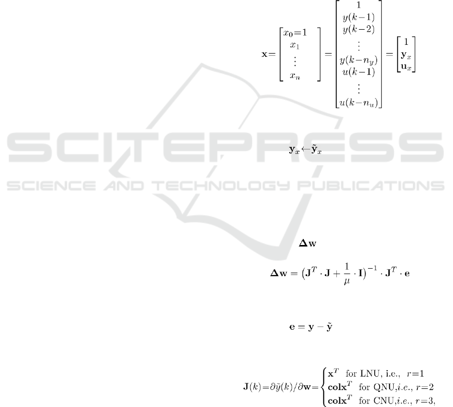
defined in Table 1, where the augmented input

vector for dynamical system approximation can be

defined in (1)and its total length is

nnn=+ + .

Recall, that y as measured one in (1) implies static a

HONU, i.e. static function mapping, because all the

values in x are measured ones.

, (1)

In order to define dynamical (recurrent) HONUs,

real y should be replaced with neural outputs, i.e.

y←



resp. in (1), so we would obtain a

recurrent neural architecture that can be more

difficult to train, but it is necessary for tuning a

controller for nonlinear dynamical systems as it is

discussed later in this paper. For batch learning for

plant identification, simple variant of Levenberg-

Marquardt algorithm can be recommended for both

static HONUs as well as for recurrent ones so the

weight updates can be calculated as follows

, (2)

where J is Jacobian matrix, I is identity matrix,

upper index

-1

stands for matrix inversion, and the

error yields . Recall that the Jacobian

matrix for static HONU , i.e. the input vector (1) with

only measured values, is as follows

(3)

where colx is a long column vector of polynomial

terms as indicated in Table 1. Then, equation (3)

shows that J is constant for all training epochs of

static HONUs (i.e. when input vector is defined as in

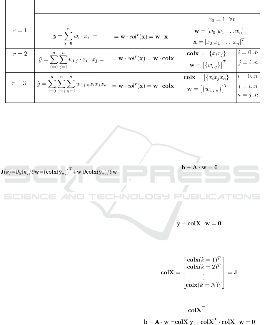
Table 1: Summary of HONUs for weakly nonlinear systems (of up to 3

polynomial order of nonlinearity).

Order of

HONU

HONU (neural output

()



)

details

Classical form of HONU = Long vector form of HONU

(LNU)

(QNU)

(CNU)

(1)) and that accelerates real time computations (esp.

when considering the HONUs are nonlinearly

mapping models yet they are linear in parameters).

The Jacobian for recurrent HONUs, i.e. when

y←



in (1), with learning formula (2), and

according to per partes derivation rule, generally

yields

,(4)

where the content of a short vector



y is apparent

from (1). Recurrent HONUs then perform more

accurate dynamical approximation of weakly

nonlinear dynamical systems from measured data

than a static HONU (as it is shown in the

experimental section); however, the Jacobian of

dynamical HONU varies in time so its rows have to

be recalculated at every time sample resulting in

varying Jacobian for every training epoch.

Further in this paper, it is shown that static HONU

can be sufficient to identify weakly nonlinear

dynamical systems so we can use a very efficient,

well converging and the most straightforward

technique of a feedback controller tuning.

3 CONJUGATE GRADIENT FOR

PLANT IDENTIFICATION

WITH HONUs

The proper plant identification from measured data

is important for further controller tuning. In case of

not well conditioned data in Jacobian, the L-M

formula (2) needs a small learning rate µ for

convergence and then this gradient method can be

slow, i.e. it may need large number of training

epochs. Nevertheless, HONUs are linear in

parameters and the CG learning can be directly

applied to HONUs as it is introduced in this section.

Recall, that CG solves the set of equations as

follows

, (5)

Where b is a column vector of constants, A is

positively semi-definite matrix, and w is a column

vector of unknowns (neural weights). Because

HONUs are linear in parameters, i.e. the Jacobian

(3) is not directly a function of weights, we can

restate the training of HONUs as follows

, (6)

where colX is defined (Bukovsky and Homma,

2016) as follows (assuming all initial conditions are

known)

, (7)

that is in fact the Jacobian of a HONU for all

training data (of total length N). Then, by

mutliplying (6) with from the left, we obtain

, (8)

so we have obtained the positive definite matrix A

and thus we can directly apply the CG learning to

both static or recurrent HONUs as follows. For the

very first epoch of training we initiate CG with

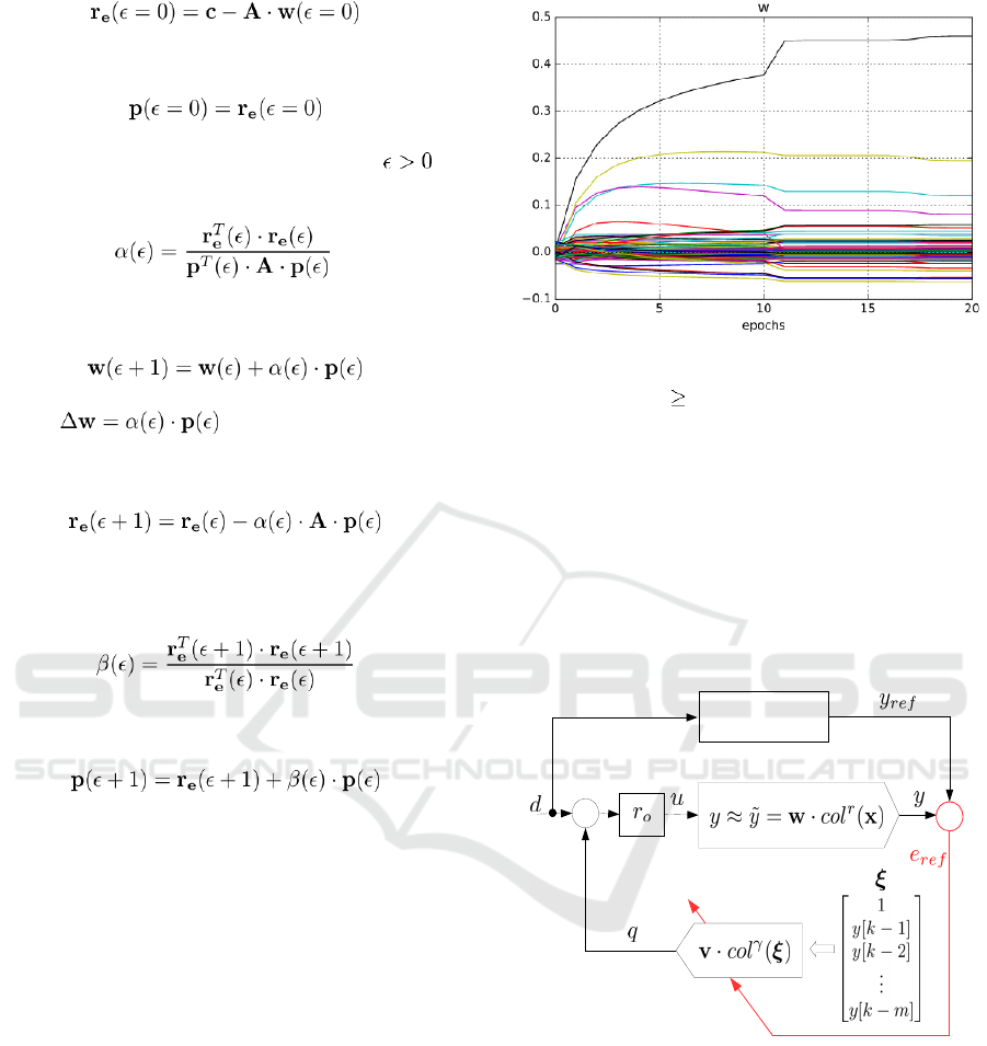
, (9)

and with

. (10)

Then for further epochs of training, i.e. for

, we

calculate parameter

, (11)

and then we can update the weights as

, (12)

where and other CG parameters for

next training epoch are then calculated or updated as

follows

, (13)

and similarly to Fletcher-Reeves nonlinear CG

method

, (14)

and finally

. (15)

This section extended the classical Conjugate

Gradient learning (as known for linear systems) to

HONUs due to their in parameter linearity. This

batch learning algorithm (9)-(15) has no adjustable

parameters except the initial neural weights and the

number of learning epochs; furthermore, the training

of both static or dynamical HONU can be rapidly

accelerated in comparison to L-M algorithm (2). As

demonstrated in experimental section in this paper, it

is suggested to use L-M learning for a few initial

training epochs and then switch for CG to rapidly

accelerate plant identification. Notice that in a

closed loop, the presented CG for HONU is not so

suitable for controller weights

training as the

symmetric positive definite matrix is not so

achievable and CG for a controller then becomes

much more complicated task. Thus L-M and CG are

both applicable to plant identification via static or

dynamic HONUs, while only L-M is the most

comprehensible training algorithm for HONUs as

controllers within the MRAC control scheme

(Figure (2))

Figure 1: Training of static CNU for system in Figure 3

starting with L-M learning accelerated with CG learning

for training epochs 10.

4 BATCH LEARNING STRATEGY

FOR CONTROL WITH STATIC

HONU AS A PLANT MODEL

The most typical control loop for SISO dynamical

systems with HONUs can be according to Figure2,

where we assume normalized (z-scored) magnitudes

plant

controller

Reference Model

Figure 2: Discrete time Model Reference Adaptive Control

(MRAC) loop with two HONUs: as plant model and as a

nonlinear state feedback controller.

of input and output variables, i.e. of d, y, and y

ref

and

where the input gain r

can be also adaptive and it

compensates for the true static gain of the controlled

plant. In our previous works on HONUs with the

MRAC control scheme in Figure 2, we have usually

identified plants with recurrent HONUs and then we

used a trained HONU as a dynamical plant model

for further controller-tuning computations, i.e.,

including for the control loop simulation with

HONU as a dynamical model of a plant. It means

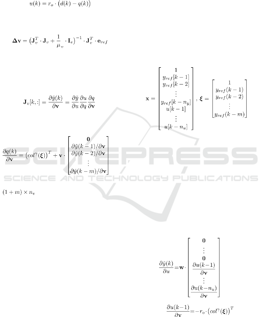
that for the control law

, (16)

the controller weights are optimized (trained) via L-

M learning rule as follows

, (17)

where the subscript v indicates it is the controller

learning rule, and where the Jacobian matrix J

involves recurrent backpropagation computations of

partial derivatives (with properly applied time

indexes as follows

, (18)

so we should calculate the Jacobian (18) recurrently

because

, (19)

where the utmost right matrix has its dimension of

, and n

denotes the total number of

neural controller weights (i.e. the lengh of v). For

the above controller training (16)-(19) (with

dynamical HONU as plant model), both the input

vectors x in (1) and

ξ in (Figure 2). Based on our

contemporary knowledge (Benes and Bukovsky,

2014; Benes et al., 2014; Bukovsky et al., 2015,

n.d.), the above control scheme with dynamic plant

HONU works very well if the dynamical HONU can

be trained to identify the plant, i.e. if the plant is not

more nonlinear than as it could be captured by the

dynamical HONU. In other words, we always

suggest to try to identify the plant with a dynamical

HONU for control tuning for MRAC approach.

Nevertheless, in case of weakly nonlinear plants, i.e.

plants that can be well identified by the dynamical

HONUs due to not too high degree of nonlinearity,

we may avoid the recurrent computations and we

can train the controller weights in much more

straightforward and computationally efficient

strategy as follows.

At the beginning of controller training and before

the plant identification, we always need a reasonable

training data, here we define the desired variable d

that we can feed into the plant to measure the

corresponding plant output data y, and we also

simulate the reference model output y

ref

. Recall that

the objective is to modify the control loop so it

adopts the reference model behavior once the

controller is properly trained. In other words, we

desire that the trained controller outputs a proper

value q so in the next corresponding future steps, the

controlled plant y matches the reference model

output y

ref

, (20)

Thus, if we feed the reference values directly into

the input vectors of plant (1) and controller

(Figure2) as in (20) i.e. we do not need to simulate

the closed loop output with a recurrent HONU

model of a plant but instead we use directly the

apriori given reference model values, then we can

update the controller weights directly and the k

row

of Jacobian (18) can be directly evaluated in (21)

where the weights w were obtained by L-M and/or

CG learning algorithm with static HONU as a plant

model. Thus, we have avoided the recurrent

computations in both plant identification as well as

controller training and the computational efficiency

and convergence of the learning is boosted.

; where (21)

However as mentioned above, the price for this

boosted controller design is that this way trained

controllers are limited to linear or weakly nonlinear

plants, i.e. to such plants for which the static HONU

sufficiently approximates the system from data

(otherwise recurrent HONU has to be used for plant

identification for the control scheme and it can be

more difficult to train dynamical HONU properly or

even impossible depending on nonlinearity of the

approximated system).

5 EXPERIMENTAL ANALYSIS

The plant dynamics was first identified from input-

output data with static HONU and another static

HONU(s) were trained as controllers (Figure 2) with

L-M training, so the recurrent computations and

plant simulation during the plant identification and

controller training were avoided. All the

computations were implemented in Python (2.7)

including the continuous time simulation of plants

and closed control loops (Scipy odeint with default

setups unless noted otherwise).

5.1 Linear Oscillating Dynamical

System

To demonstrate the efficiency of the proposed

control approach with HONU for oscillatory linear

dynamical systems, a SISO plant defined with the

Laplace transfer function is chosen as follows

, (22)

where s is the Laplace operator. The training data

were simulated with sampling

[time unit] and

its dynamics was approximated with a single static

LNU (i.e. HONU r=1, n

=5, n

=5, µ=0.1, 300

training epochs of L-M training) for the same

constant sampling. To enhance the controller

performance for this dynamical system with

complex conjugate poles and zeros, two parallel

LNUs were used as a controller to enhanced control

performance as introduced recently in (Bukovsky et

al., n.d.). Recall that in such case, the controller

consisted of two summed LNUs so the control law

(16) yielded

, (23)

where q

and q

are outputs of two parallel LNUs

(while only a single one is shown in Figure 2). Both

controller LNUs were trained with L-M learning

with input vector setups m

=5, m

=5, and with the

same learning rate

= for the weights and for

within 30 training epochs. The performance of

the trained controller is shown in Figure 4.

5.2 Weakly Nonlinear System

As an example of a weakly nonlinear system, the

second-order dynamics plant is chosen as defined in

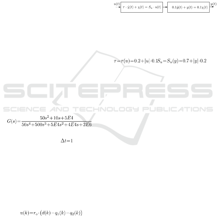
Figure 3,

Figure 3: A weakly nonlinear plant where ()u

ττ

= and

()

SSy= are nonlinear functions (24).

where the time constant τ and the static gain S

the first subsystem are nonlinear functions as

follows

.(24)

The continuous-time plant (to obtain “measured”

data) and the continuous control loop were simulated

with sampling Δt=0.01 [time unit] with forward

Euler method. The plant was identified from

“measured” data with static CNU (HONU r=3)

with setups n

=3, n

=3 and with initial 10 epochs of

L-M with µ=0.01 followed with 10 epochs of CG for

accelerated learning (see the accelerated

convergence in Figure 1). Further a single CNU as a

controller (as in Figure 2) with setup m=2 and also

were trained by L-M (10 epochs, µ

=1E6). The

sampling of plant identification and controller

actuation was here Δt

HONU

=0.5 [time unit]. The

performance of the trained control loop compared to

the plant without a controller is shown in Figure 5.

6 DISCUSSION

To discuss the limitations of HONUs of up to 3

polynomial order, i.e. r ≤ 3, as we have investigated

them for nonlinear dynamical systems up to now,

let’s discuss identification and control of an inverted

pendulum model (25) with HONUs in this section.

The model (23) is adopted from (Liu and Wei,

2014); however, it is modified with increased

friction to at least stabilize the system first to obtain

training data for plant identification. It should be

highlighted, that the MRAC control approach

depends on plant model, here learned from training

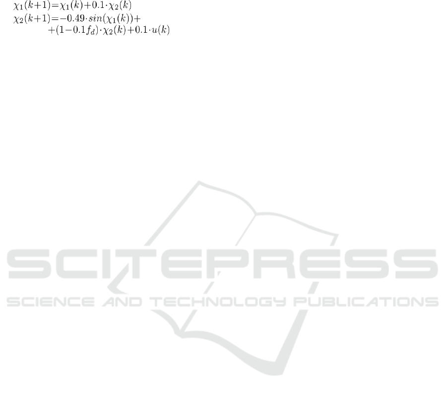
data, and such data can not be usually obtained from

unstable systems. The modified (stabilized) discrete

time inverted pendulum model is then as follows

(25)

where the measured output is simulated as y=χ

=0.6 is the friction and u is control input. A

successful setup for at least imperfect control of this

plant (see Figure 6) was found at doubled sampling

with static CNU for identification (r=3, n

=4,

trained with 20 epochs of L-M (µ=1) followed with

20 epochs of CG ) and two parallel static HONUs

(LNU and CNU) as a controller, as discussed in

subsection 5.1 (23), both with m=4 and with 30

epochs of L-M training (µ

=1). The successful setup

for control of this more strongly nonlinear plant was

not so trivial to find as it was for the previous two

weakly nonlinear plants. The control result for (25)

is shown in Figure 6.

7 CONCLUSIONS

In this paper, we have presented MRAC control

strategy with purely static HONUs that avoids

recurrent computations and thus improves

convergence of controller training. As an aside, the

Conjugate Gradient was presented for HONUs as it

can accelerate plant identification with HONUs.

This adaptive control technique is easy to implement

and it was shown working for weakly nonlinear

dynamical systems, i.e. such systems that can be

well approximated with HONUs of appropriate

polynomial order (here < 3). Investigating this

straight control approach with HONUs for strongly

nonlinear systems is still a challenge.

ACKNOWLEDGEMENT

The work was supported by the College of

Polytechnics, Jihlava, Czech Republic, and by the

Japanese JSPS KAKENHI Grant Number 15J05402.

Special appreciation goes to people that have been

developing Python, LibreOffice and other useful

open-source SW.

REFERENCES

Benes, P., Bukovsky, I., 2014. Neural network approach to

hoist deceleration control, in: 2014 International Joint

Conference on Neural Networks (IJCNN). Presented

at the

2014 International Joint Conference on Neural

Networks (IJCNN), pp. 1864–1869

. doi: 10.1109/

IJCNN.2014.6889831

Bukovsky, I., Benes, P., Slama, M., 2015. Laboratory

Systems Control with Adaptively Tuned Higher Order

Neural Units, in: Silhavy, R., Senkerik, R., Oplatkova,

Z.K., Prokopova, Z., Silhavy, P. (Eds.),

Intelligent

Systems in Cybernetics and Automation Theory,

Advances in Intelligent Systems and Computing.

Springer International Publishing, pp. 275–284

Bukovsky, I., Benes, P.M., Vesely, M., Pitel, J., Gupta,

M.M., n.d. Model Reference Multiple-Degree-of-

Freedom Adaptive Control with HONUs, in:

The 2016

International Joint Conference on Neural Networks.

Presented at the IEEE WCCI 2016, IEEE, Vancouver

Bukovsky, I., Homma, N., 2016. An Approach to Stable

Gradient-Descent Adaptation of Higher Order Neural

Units.

IEEE Trans. Neural Netw. Learn. Syst. PP, 1–

13.

doi:10.1109/TNNLS.2016.2572310

Dai, Y.H., Yuan, Y., 1999. A Nonlinear Conjugate Gradient

Method with a Strong Global Convergence Property.

SIAM J. Optim. 10, 177–182. doi: 10.1137/

S1052623497318992

Elbuluk, M. E., Tong, L., Husain, I., 2002. Neural-

Network-Based Model Reference Adaptive Systems

for High-Performance Motor Drives and Motion

Controls.

IEEE Trans. Ind. Appl. 38, 879–886.

doi:10.1109/TIA.2002.1003444

El-Nabarawy, I., Abdelbar, A. M., Wunsch, D.C., 2013.

Levenberg-Marquardt and Conjugate Gradient

methods applied to a high-order neural network. IEEE,

pp. 1–7.

doi:10.1109/IJCNN.2013.6707004

García, C. E., Prett, D. M., Morari, M., 1989. Model

predictive control: Theory and practice — A survey.

Automatica 25, 335–348. doi: 10.1016/0005-

1098(89)90002-2

Ivakhnenko, A. G., 1971. Polynomial Theory of Complex

Systems. IEEE Trans. Syst. Man Cybern. SMC-1,

364–378. doi:10.1109/TSMC.1971.4308320

Kosmatopoulos, E. B., Polycarpou, M. M., Christodoulou,

M.A., Ioannou, P.A., 1995. High-order neural network

structures for identification of dynamical systems.

IEEE Trans. Neural Netw. 6, 422–431.

doi:10.1109/72.363477

Ławryńczuk, M., 2009. Neural Networks in Model

Predictive Control, in: Nguyen, N. T., Szczerbicki, E.

(Eds.), Intelligent Systems for Knowledge

Management.

Springer Berlin Heidelberg, Berlin,

Heidelberg, pp. 31–63.

doi: 10.1007/978-3-642-

04170-9_2

Liu, D., Wei, Q., 2014. Policy Iteration Adaptive Dynamic

Programming Algorithm for Discrete-Time Non-linear

Systems.

IEEE Trans. Neural Netw. Learn. Syst. 25,

621–634.

doi:10.1109/TNNLS.2013.2281663

Madan M. Gupta, Ivo Bukovsky, Noriyasu Homma, Ashu

M. G. Solo, Zeng-Guang Hou, 2013.

Fundamentals of

Higher Order Neural Networks for Modeling and

Simulation, in: Ming Zhang (Ed.), Artificial Higher

Order Neural Networks for Modeling and Simulation.

IGI Global, Hershey, PA, USA, pp. 103–133.

Morari, M., H. Lee, J., 1999. Model predictive control:

past, present and future. Comput. Chem. Eng. 23, 667–

682.

doi:10.1016/S0098-1354(98)00301-9

Narendra, K. S., Valavani, L. S., 1979. Direct and indirect

model reference adaptive control. Automatica 15, 653–

664.

doi:10.1016/0005-1098(79)90033-5

Nikolaev, N. Y., Iba, H., 2006. Adaptive learning of

polynomial networks genetic programming,

backpropagation and Bayesian methods.

Springer,

New York.

Osburn, P. V., 1961. New developments in the design of

model reference adaptive control systems.

Institute of

the Aerospace Sciences.

Parks, P. C., 1966. Liapunov redesign of model reference

adaptive control systems

. Autom. Control IEEE Trans.

On 11, 362–367.

Taylor, J. G., Coombes, S., 1993. Learning Higher Order

Correlations.

Neural Netw 6, 423–427. doi: 10.1016/

0893-6080(93)90009-L

Tripathi, B. K., 2015. Higher-Order Computational Model

for Novel Neurons, in: High Dimensional Neurocom-

puting. Springer India, New Delhi, pp. 79–103.

Wang, F.-Y., Zhang, H., Liu, D., 2009. Adaptive Dynamic

Programming: An Introduction. IEEE Comput. Intell.

Mag. 4, 39–47.

doi:10.1109/MCI.2009.932261

Wang, X., Cheng, Y., Sun, W., 2007. A Proposal of

Adaptive PID Controller Based on Reinforcement

Learning. J.

China Univ. Min. Technol. 17, 40–44.

doi:10.1016/S1006-1266(07)60009-1

Zhu, T., Yan, Z., Peng, X., 2017. A Modified Nonlinear

Conjugate Gradient Method for Engineering

Computation. Math. Probl. Eng. 2017, 1–11.

doi:10.1155/2017/1425857

APPENDIX

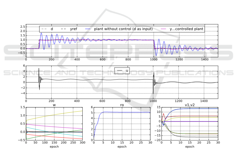
Figure 4: Results for linear oscillatory plant (22) via static LNU as a plant model (trained via L-M) and two parallel LNUs

as a feedback controllers (trained via L-M); the control loop output follows the desired unit steps reference signal (yref) (the

upper plot), the control input (2

from top), bottom axes shows training by L-M batch learning of static LNU for plant

(bottom left), input gain (middle), and static LNU as controller (bottom right).

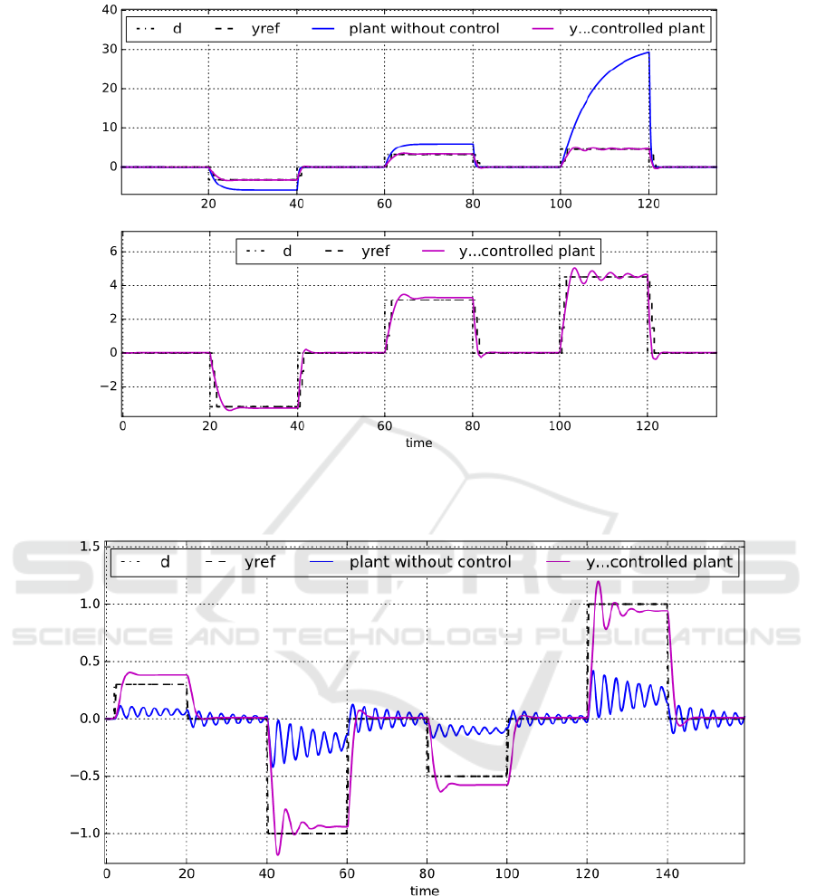
Figure 5: Results for control of weakly nonlinear dynamical system (Subsection 5.2) with variable time constant and static

gain (24), static CNU as a plant model (trained via L-M + CG, Figure 1) and static CNU controller (via L-M) (the bottom

axes show the detail of the desired behavior with the trained control loop output).

Figure 6: Control of plant (25); with the increasing desired value (dashed), the accurate control is more difficult to achieve

as the sinusoidal nonlinearity becomes stronger with increasing magnitude of desired value, so it demonstrates current

limits and challenges of the identification and control of strongly nonlinear systems with HONUs.