
Detecting and Assessing Contextual Change in Diachronic Text
Documents using Context Volatility
Christian Kahmann, Andreas Niekler and Gerhard Heyer
Leipzig University, Augustusplatz 10, 04109 Leipzig, Germany
Keywords:
Context Volatility, Semantic Change.
Abstract:
Terms in diachronic text corpora may exhibit a high degree of semantic dynamics that is only partially captured
by the common notion of semantic change. The new measure of context volatility that we propose models the
degree by which terms change context in a text collection over time. The computation of context volatility for
a word relies on the significance-values of its co-occurrent terms and the corresponding co-occurrence ranks
in sequential time spans. We define a baseline and present an efficient computational approach in order to
overcome problems related to computational issues in the data structure. Results are evaluated both, on syn-
thetic documents that are used to simulate contextual changes, and a real example based on British newspaper
texts. The data and software are avaiable at https://git.informatik.uni-leipzig.de/mam10cip/KDIR.git.
1 INTRODUCTION
When dealing with diachronic text corpora, we fre-
quently encounter terms that for a certain span of time
exhibit a change of linguistic context, and thus in
the paradigm of distributional semantics exhibit a
change of meaning. For applications in information
retrieval and machine learning tasks this causes prob-
lems because terms then are not unambiguous, hin-
dering the task of retrieving, or structuring, relevant
documents or information. However, understanding
semantic change can also be a research goal on its
own, such as work in historical semantics (Simpson
et al., 1989), or in the digital humanities where se-
mantic change has been used as a clue to better un-
derstand political, scientific, and technical changes,
or cultural evolution in general (Michel et al., 2011;
Wijaya and Yeniterzi, 2011). In information retrieval,
finding terms that significantly change their meaning
over some period of time can also be a key to ex-
ploratory search (Heyer et al., 2011).
While there is plenty of work on how to detect
and describe semantic change of particular words,
for example “gay”, “awful”, or “broadcast” in En-
glish between 1850 and 2000 (Hamilton et al., 2016,
cf.) by highlighting the differences in context as de-
rived by co-occurrence analysis (Jurish, 2015, cf.) or
topic models (J
¨
ahnichen et al., 2015, e.g.), it is still
an open question of how to identify those terms in a
diachronic collection of text that undergo by some
degree a change of context, and thus exhibit a se-
mantic change in the paradigm of distributional se-
mantics. In what follows, we present context volatil-
ity as a new and innovative measure that captures a
term’s rate of contextual change during a certain pe-
riod of time. The proposed measure allows to specify
the degree of a term’s contextual changes in a doc-
ument collection over some period of time, irrespec-
tively of the amount of text. This way we are able
to identify terms in a diachronic corpus of text that
are semantically stable, i.e. that undergo little or no
changes in context, as well as terms that are seman-
tically volatile, i.e. that undergo continuous or rapid
changes in their linguistic context. Often, semanti-
cally volatile terms are highly controversial, such as
“Brexit“ in the 2016 British public debate. A term’s
context volatility complements its frequency, a feature
that is of particular interest when we are interested in
detecting weak signals, or early warnings, in the tem-
poral development of a corpus related to low frequent
terms indicating subsequent semantic change. Con-
text volatility is related to the notion of volatility in fi-
nancial mathematics (Taylor, 2007), and we can draw
a rough analogy that just like the rate of change in the
price of a stock is an indication of risk, a high degree
of context volatility of a term is an indication that the
fair meaning of a term is still being negotiated by the
linguistic community.
We begin in section 2 by showing how our ap-
proach differs from other procedures in the spirit of
Kahmann C., Niekler A. and Heyer G.
Detecting and Assessing Contextual Change in Diachronic Text Documents using Context Volatility.
DOI: 10.5220/0006574001350143
In Proceedings of the 9th International Joint Conference on Knowledge Discovery, Knowledge Engineering and Knowledge Management (KDIR 2017), pages 135-143
ISBN: 978-989-758-271-4
Copyright
c
2017 by SCITEPRESS – Science and Technology Publications, Lda. All rights reserved

distributional semantics. We then explore and eval-
uate different forms of contextual change and iden-
tify computational problems that arise when applying
context volatility to diachronic text corpora. By eval-
uating the basic intuition and strategies to overcome
the difficulties we shall then present in section 3 an
approach which robustly calculates context volatility
without any statistical bias, and in section 4 introduce
a novel algorithm which avoids sparsity problems on
diachronic corpora, the MinMax-algorithm. To eval-
uate the measure, we apply the algorithm to a syn-
thetic data set in section 5, based on a distinction be-
tween three cases of how the context of a word may
change, viz. (1) a change in the probability of co-
occurring terms, (2) the appearance of new contexts,
and (3) the disappearance of previous contexts. Fi-
nally we apply our measure to real life data from the
Guardian API and illustrate its usefulness in contrast
to a purely frequency based approach with respect to
the term “Brexit”.
2 RELATED WORK
Several studies address the analysis of variation in
context of terms in order to detect semantic change
and the evolution of terms. Three different areas to
model contextual variations can be distinguished: (1)
methods based on the analysis of patterns and linguis-
tic clues to explain term variations, (2) methods that
explore the latent semantic space of single words, and
(3) methods for the analysis of topic membership. (Ja-
towt and Duh, 2014) use the latent semantics of words
in order to create representations of a term’s evolu-
tion which is a similar information as used in context
volatility. The approach models semantic change over
time by setting a certain time period as reference point
and comparing a latent semantic space to that refer-
ence over time. (Fernndez-Silva et al., 2011; Mitra
et al., 2014) or (Picton, 2011) look for linguistic clues
and different patterns of variation to better understand
the dynamics of terms. The popular word2vec model
has also been utilized for tracking changes in vocab-
ulary contexts (Kim et al., 2014; Kenter et al., 2015).
Both word2vec-based approaches use references in
time or seed words to emphasize the change but do
not quantify it independently to the reference. (Kim
et al., 2014) add the quantity of the changes through-
out growing time windows towards a global context
representation but do not examine the possibility of
detecting different phases in the intensity of change
whereas (Kenter et al., 2015) produce changing lists
of ranked context words w.r.t. the seed words. One
major concern in suing the word2vec approaches is
the fact that those models require large amounts of
text. Both described approaches fulfill this require-
ment by a workaround to artificially boost the amount
of data. This influences the ability to quantify and de-
scribe contextual changes according to the observable
data. Assuming a Bayesian approach, topic modeling
is another method to analyze the usage of terms and
their embeddedness within topics over time (Blei and
Lafferty, 2006; Zhang et al., 2010; Rohrdantz et al.,
2011; Rohrdantz et al., 2012; J
¨
ahnichen, 2016). How-
ever, topic model based approaches always require an
interpretation of the topics and their context. In ef-
fect, the analysis of a term’s change is relative to the
interpretation of the global topic cluster, and strongly
depends on it. In order to identify contextual varia-
tions, we also need to look at the key terms that drive
the changes at the micro level. Context volatility dif-
fers from previous work in its purpose because it does
not start with a fixed set of terms to study and trace
their evolution, but rather detects terms in a collec-
tion of documents that may be indicative of contex-
tual change for some time. The notion of context
volatility is introduced in (Heyer et al., 2009; Holz
and Teresniak, 2010; Heyer et al., 2016). The respec-
tive works present single case studies to evaluate the
plausibility of the proposed measure. Several nega-
tive effects in the data are not discussed and evalu-
ated. For example, the appearance of new contexts
or the absence of certain word associations in sin-
gle time slices cause gaps in the co-occurrence rank
statistics which were ignored in those works. The
measure determines the quantity of contextual change
by observing the coefficient of variance in the ranks
for all word co-occurrences throughout time. Addi-
tionally, it does not use latent representations but the
co-occurrence information itself without any smooth-
ing. The information of temporarily non-observable
co-occurrences is present and can be used for the de-
termination of contextual change directly. In section 3
we take up on those effects that directly influence the
procedure and define alternative approaches to over-
come associated problems. In sum, while related
work on the dynamics of terms usually starts with a
reference (like pre-selected terms, reference points in
time, some pre-defined latent semantics structures, or
given topic structures), context volatility aims at auto-
matically identifying terms that exhibit a high degree
of contextual variation in a diachronic corpus regard-
less of some external reference or starting point. The
measure of context volatility is intended to support
exploratory search for central terms
1
in diachronic
1
The notion of centrality of terms is used in (Picton,
2011). It captures the observation that central terms simul-
taneously appear or disappear in a corpus when the key as-

corpora, in particular, if we want to identify peri-
ods of time that are characterized by substantial se-
mantic transformation. However, we do not claim
that the measure quantifies meaning change or seman-
tic change, the measure quantifies the dynamics of a
term’s contextual information within a diachronic cor-
pus.
3 DEFINITION OF CONTEXT
VOLATILITY
The computation of context volatility is based on
term-term matrices for every time slice derived from
a diachronic corpus (Heyer et al., 2016). Those matri-
ces hold the co-occurrence information for each word
w in a time slice t. One can use different significance
weights based on the co-occurrence counts such as the
log-likelihood-ratio, the dice measure or the mutual
information to represent the co-occurrences (Bordag,
2008). First, the corpus is divided into sets of docu-
ments belonging to equal years, months, weeks, days
or even hours and minutes to define the time slices
t. The set of all time slices is T . It is necessary to
determine for every word w of the vocabulary V and
every time slice t the co-occurrences w∗, e.g. a term-
term matrix C
t
with the co-occurrence counts. The
matrix has dimension V ×V . Based on the counts in
C
t
a significance-weight can be calculated on all word
pairs which results in a term-term matrix of signif-
icant co-occurrences S
t
. The significance-values for
the co-occurrences of a word w in t are sorted to as-
sign a ranking to the co-occurrences of a word. For
every word which co-occurs with w in t this ranking
may differ in the time slices or the ranking can’t be
applied if this very co-occurrence is not observable.
The ranks are stored in a matrix R
t
. Based on con-
secutive time stamps the ranks for every word pair in
all R
w,w∗,t
build a sequence. The transition of a word
pairs ranking through the time slices is quantified by
the coefficient of variance on the ranks. It is possi-
ble to perform this calculation only on a history h of
time slices which gives the variance in the ranking
of a word pair for a shorter time span. The context
volatility for a word w in t is then the mean of all
rank variances from the word pairs w, w*. Note, that
not all combinations in w, w* have a count > 0 in all
time slices simply because not every word co-occurs
with every other word all the time. There are words
which never occur together with w or just in some
time slices. We therefor define the basic measure of
sumptions, or consensus, amongst the stakeholders of a do-
main change
context volatility of a term as an averaged operation
cv(C
w,i
, h) on all co-occurences of w where C
w,i
is the
i
th
co-occurrence of w. In the basic setting the mean
is build over all co-occurrences w* of w which can be
observed in at last 1 time stamp in h. Precisely, we
can define the final calculation of the volatility for h
as
CV
w,h
=
1
kC
w,h
k
∑
i
cv(C
w,i
, h), (1)
with kC
w,h
k the number of co-occurrences on w which
could be observed in h. For consecutive histories the
context volatility of w forms a time series where each
data point contains the context volatility at a time slice
t for a given history h. This represents the mean con-
text volatility for all contextual information about a
word and we get an average change measure for the
co-occurrences. Informally, context volatility com-
putes a term’s change of context by averaging the
changes in its co-occurrences for a defined number
of time slices. Alternatively, h could be set to all time
slices in T to produce a global context volatility for
the words in a diachronic text source.
3.1 Limitations
So far the main limitation of context volatility has
been an adequate handling of gaps. When applying
context volatility as described in (Holz and Teresniak,
2010) it can be shown that there are many cases for
which a co-occurrence of 2 words at a specific point of
time not only changes in usage frequency. The effect
could be observed in cases for which new vocabulary
is associated with a given word w in diachronic cor-
pora or some contexts are temporarily not used. This
does not necessarily mean that the absence of a con-
text introduces a lasting change to the semantic mean-
ing of a word. But both cases contain important infor-
mation about the dynamics in the contextual embed-
ding of a word. Thus, the resulting gaps in the rank se-
quence of diachronic co-occurrences for a word must
be handled accordingly to prevent a bias. Different
strategies for the handling of those gaps seem plau-
sible. For example, consider the situation where we
calculate the variance of 10 consecutive ranks, e.g. h
is set to 10 time slices, of a co-occurring word which
is given by R
w,i,h
= 1, X, 2, X, 3, X, 4, X, 5, X. The X
represents a gap, e.g. a co-occurrence count of 0 in
the according time slice. If the volatility of this pro-
gression should be calculated as in (Holz and Teres-
niak, 2010) we would calculate the coefficient of vari-
ation of all ranks which are observable. In the ex-
periments the authors used a very large corpus with a
large h and the influence of the gaps is presumed to
produce a small bias. However, for smaller corpora

or smaller amounts of documents for a time slice we
can’t ignore the influence of such decisions. Often, a
co-occurrence can only be observed in a minority of
the time slices if, for example, the corpus is reduced
to a set of documents containing a specific topic. Fol-
lowing the definition of (Holz and Teresniak, 2010)
we set
cv(C
w,i
, h) =
σ(R
w,i,h
)
¯
R
w,i,h
. (2)
Likewise, we can use the significance-values for co-
occurring terms directly and set
cv(C
w,i
, h) = σ(S
w,i,h
), (3)
where σ(S
w,i,h
) is the standard deviation of the i
th
co-
occurrence significances of w in the history h. We use
the standard deviation since the significance-values
are not linearly distributed and a major amount of co-
occurrences has very little significance-values. Using
the coefficient of variance would produce large values
in changes of small significances which is an unde-
sired behavior.
To carry out this calculations in a similar man-
ner like (Holz and Teresniak, 2010) only values of
R
w,i,h
are included which can be observed in the data,
e.g. R
w,i,h
= 1, 2, 3, 4, 5. We do not include the
non-observable co-occurrences with 0 or the maxi-
mum possible rank, e.g. the count of all possible co-
occurrences or the vocabulary, to fill the gaps because
this introduces an undesired bias. A better strategy to
handle the non-observable ranks is to set the missing
co-occurrence in t by other information. We calcu-
late all co-occurrence significances on all documents
on all time slices first, in order to have a “global“ co-
occurrence statistic S
G
. If a significance value in a
time stamp S
w,i,t
cannot be observed we set this value
to S
G
w,i
if this significance is greater than 0, e.g. the
co-occurrence can be observed in some time stamp in
T but not in all. This deletes the gaps and introduces a
global knowledge about the contexts. Co-occurrences
which are new or emerging or just observable in some
time stamps are somehow of higher significance in the
time stamp but of lower significance w.r.t. the whole
corpus. This procedure prevents a bias and numerical
problems with missing ranks or significances. How-
ever, the dynamics in the co-occurrence statistics are
still determinable. In section 5 we evaluate the base-
line method by using the ranks and measure their co-
efficient of variance by ignoring missing information
(Baseline). Additionally, we test the same setup using
the significances directly (Sig). Both setups are eval-
uated once again with beforehand added global co-
occurrence information(GlobalBaseline, GlobalSig).
4 MINMAX-ALGORITHM
In contrast to the notion of context volatility, where
the gaps were either not used at all or replaced by
global information, the MinMax-algorithm does use
the gap information itself. The difference d in the
ranks of a co-occurrence w, w* is measured from time
slice to time slice separately, then summed up and di-
vided by the number of time slices considered. This
results in a mean distance between the ranks of the
time slices w.r.t. w and h. A major distinction is the
introduction of 2 different ranking functions (formula
4 and 5) when setting the ranks for all co-occurences
w, w∗ in a time slice t. We apply both formulas to
all observable co-occurrences resulting in 2 ranks per
co-occurrence. Formula 4 applies the ranks decreas-
ing from the maximum number of co-occurrences w
has in a time slice considered in h. Words w∗ with
significance-values of 0, e.g. gaps, share rank 0. In
formula 5 the ranks are assigned decreasing from the
number of co-occurrences w has in time slice t. Sig-
nificances with value 0 again share rank 0. In the fol-
lowing equations R
w,w∗,t
is the list of co-occurrence
ranks for word w w.r.t. time slice t and R
w,i,t
the
rank of the i
th
co-occurrence for w w.r.t. t. The
quantity max(R
w,w∗,1...h
) is the maximum rank an ob-
servable co-occurrence of w can take in a history h,
e.g. the maximum number of co-occurrences of w
amongst the time slices included in h. Additionally,
this quantity is utilized to normalize the determined
ranks in the interval [0,1]. The normalization re-
moves the strong dependence towards a high number
of co-occurrences because the higher the number of
co-occurrences, the more likely it is to see a higher
absolute change for the ranks. This enables the com-
parison of words with big differences in their frequen-
cies and with that in their number of co-occurrences.
R
¬0
(R
w,w∗,t
) =
max(R
w,w∗,1...h
) + 1 − R
w,i,t
max(R
w,w∗,1...h
)
(4)
R
0
(R
w,w∗,t
) =
max(R
w,w∗,t
) + 1 − R
w,i,t
max(R
w,w∗,1...h
)
(5)
Consequently, besides having an absolute maximum
(rank for highest significance) we now confirm having
an absolute minimum (rank 0) over all time slices as
well. The gap-information is used directly because
when new words appear, we are able to measure the
distance between rank 0 and the relative rank a new
appearing word has in t + 1. The ranks of formula 4
are used when neither of the 2 consecutive entries to
calculate d represent a gap (R
¬0
). When either one or
both regarded entries represent a gap we use the ranks
determinded by formula 5 (R
0
). We can summarize
the procedure of calculating the mean distance of all

w, w* concurrent words to
CV
w,h
=
1
kC
w,h
k · (h − 1)
kC
w,h
k
∑
i=1
h−1
∑
t=1
cv(C
w,i,h
) (6)
with cv(C
w,i,h
) =
(
| R
0
(R
w,t,i
) − R
0
(R
w,t+1,i
) | if a
| R
¬0
(R
w,t,i
) − R
¬0
(R
w,t+1,i
) | if b
(7)
where condition a : R
w,t,i
∨ R
w,t+1,i
= 0 and b : R
w,t,i
∧
R
w,t+1,i
= ¬0.
5 EVALUATION USING A
SYNTHETIC DATASET
There is no gold standard to validate the quantity of
contextual change. Such being the case, we are uti-
lizing a synthetic data set in which we can manip-
ulate the change of a word’s context in a controlled
way. We simulate different situations, where the rate
of context change follows clearly defined target func-
tions. We apply the procedures presented in section 3
and 4 to the synthetic data set and compare the results
to the target functions we aimed for.
5.1 Creating a Synthetic Data Set
The creation of the data set follows 2 competing
goals. On one hand we want our data set to be as close
to an authentic data set as possible. Therefore, our
synthetic data set should be Zipf-distributed in word-
frequency which induces noisiness. On the other hand
the context volatility that follows the target functions
has to be measurable. Hence, when manipulating the
context of a word over time, we can’t ensure to not
infringe the regulations for a Zipf-distribution. We
create a data set that is somewhat Zipf-distributed but
still contains the signals we want to measure (figure
1) as a trade-off between signal and noise. The cre-
ation of the data set requires a number of time stamps
(100), a vocabulary size (1000), the mean-quantity of
documents per time stamp (500) and a mean amount
of words per document (300). To simulate the Zipf-
distribution, we create a factor f
i
Zip f
=
1000
i
, which
assigns to every word w
1,...,1000
a value indicating a
word count. The factors of counts can be normal-
ized to probability distributions when constructing the
documents. We also define 7 factors f
1,...,7
respon-
sible for simulating a predefined contextual change.
The values for 7 words w
51,...,57
are set to 0 in the
Zipf-factor ( f
51,...,57
Zip f
= 0) because they’ll get boosted
in the respective factors f
1,...,7
and serve as reference
on which we evaluate the contextual change. Addi-
tionally, we designate the first 50 words in the artifi-
cial vocabulary, e.g. w
1,...,50
, to act as stopwords. In
each of the 7 factors we set 150 randomly chosen non-
stopwords to simulate an initial context w, w∗ and we
assign some high values according to ∼ N (75, 25).
The values for the reference words w
51,...,57
in their
associated factor is fixed to 200. All other words
in a factor get a value close to 0 (0.1). The 150
other words (w, w∗) in each factor represent the ini-
tial words that are very likely to form co-occurrences
with their respective fixed word at the first time stamp.
The simulation of the contextual change now influ-
ences the distribution of the 7 factors f
1,...,7
from time
stamp to time stamp. Thereby, each factor context is
modified following 1 of the target functions triangle
( f
1
), sinus ( f
2
), constant 0 ( f
3
), slide ( f
4
), half cir-
cle ( f
5
), hat ( f
6
) and canyon ( f
7
). Illustrations of the
functions are located in the appendix. Having initi-
ated all factors, the words for every document refer-
ring to the first time stamp are sampled. We use a
uniform-distribution to choose 1 factor j among f
1,...,7
for every document. Next, we collect a preselected
amount of samples for the document using a multino-
mial distribution
p(w
i
) =
f
Zip f
(w
i
) + f
j
(w
i
)
∑
V
j
f
Zip f
(w
j
) + f
j
(w
j
)
(8)
over the whole vocabulary. By adding together the the
Zipf-factor and the sampled factor j we are adding ar-
tificial noise to the creation of the documents. We
could set the influence of the Zipf-factor separately.
But a higher proportion leads to more noise inter-
fering the context signals. The result is a bag of
words constituting each document in the first time
stamp. To proceed to the next time stamp the fac-
tors f
1,...,7
have to be altered to simulate contextual
change. The target functions control the amount of
change in their corresponding factors in dependence
to the time stamp to influence the sampling outcome,
and consequently the context of the reference words.
Note, the value for the context word in the respective
factor stays the same and must stay 0 in all other fac-
tors (e.g. f
w
51
1
= 200, f
w
51
2,...,7
= 0). Besides the defini-
tions of functions to control the amount of contextual
change we identify 3 different cases how the context
of a word can be influenced.
i. Exchange the Probability for Co-occurring
Terms: We model this by taking 2 words from the
co-occurrences w, w∗ in a factor and swap their
probabilities. This leads to a change of their like-
lihood to be sampled in the same documents like
their context word.
ii. Appearance of New Contexts: To address this,
we select 1 word in a factor that has a value close
to 0 and replace it with a high value. As a conse-
quence, when sampling the words, we will likely
see a ”new” word w.r.t. the context word of a fac-
tor.
iii. Disappearance of Contexts: We change the
probability value of a co-occurring word (high
value) close to 0. This will likely cause this word
to not appear anymore along with a context word.
In order to create the documents for the following
time stamps, the factors f
t
1,...,7
are influenced in de-
pendence to the the factors of the former time stamp
(t − 1) w.r.t a target function.
f
t
j
∼ change
targetF unction
( f
t−1
j
) (9)
For example if f
1
is following the triangle function,
for t < 50 the number of exchanged contexts can
be determined by the time stamp index t. For time
stamps t > 50 the number of exchanges is determined
100 −t. With the updated factors the succeeding time
stamps can be sampled until every document in T is
filled. The final data set for the 7 target functions and
all 3 options for contextual change is distributed as
shown in figure 1. The data set is not exactly Zipf-
distributed because of the forced co-occurrence be-
havior.
2e+03 1e+04 5e+04 2e+05 1e+06
1 5 10 50 100 500 1000
frequency
words
Figure 1: Synthetic dataset with double log scale.
5.2 Results of Evaluation
We created 3 different data sets to test strengths and
weaknesses of the algorithms. In the first data set (A)
all 3 described cases of context change are included
(case i., ii., iii.). The second data set (B) is built by
only changing the probability values of already co-
occurring terms (case i.). In the third data set (C) we
deploy the options appearance of new co-occurrences
(case ii.) and disappearance of known co-occurrences
(case iii.). We use cases (ii.) and (iii.) in the same
amount for the data sets A and C, so the quantity of
co-occurrences for the respective context words stays
0.0 0.2 0.4 0.6 0.8 1.0
0 20 40 60 80 100
context volatility
time
targetfunction
minmax
globalsig
Figure 2: Results for MinMax and GlobalSig on first data
set.
constant. In data set C we refused to add the Zipf-
factor, because it interferes the forced co-occurrence
gap-effect which we intend to simulate by this config-
uration. We applied the context volatility measures to
all 3 data sets using a span of h = 2. In the interest of
a quantifiable comparison we normalized over all re-
sults (all 3 data sets) for every context volatility mea-
sure. We assess the performance of the measures by
using the mean distance between the calculated con-
text volatility and the intended target functions of the
7 context words. An example how the measures ap-
proximate the target function can be seen in figure 2.
Table 1: Results using all 3 synthetic data sets; for every
method and every data set we calculated the mean distance
over all 7 target functions.
A B C Mean
Baseline 0.25 0.11 0.29 0.217
GlobalBaseline 0.35 0.18 0.26 0.263
Sig 0.30 0.14 0.10 0.180
GlobalSig 0.22 0.25 0.08 0.183
MinMax 0.24 0.12 0.18 0.180
All calculation methods are able to detect the
function signals for data set A which sends the
strongest signals (table 1). The GlobalSig method
slightly outperforms all other methods in this setting.
The loss of information that occurs when transfer-
ring the significances to ranks might be one cause of
the overall worse performance of the baseline meth-
ods, and a opportunity to further improve the MinMax
method. When using data set B the MinMax- and the
Baseline-algorithm perform best. Context changes
where new co-occurrences appear and known disap-
pear (C), again, is best captured by methods based
on significances. The third data setting (C without
usage of f
Zip f
) forced the measurements to handle
gap-entries and the inability of the Baseline-method
in this concern is revealed. The produced results in-
clude the fact that the context words w
51,...,57
stay
constant in frequency in all time slices. Under this
condition the algorithms Sig, GlobalSig, and Min-
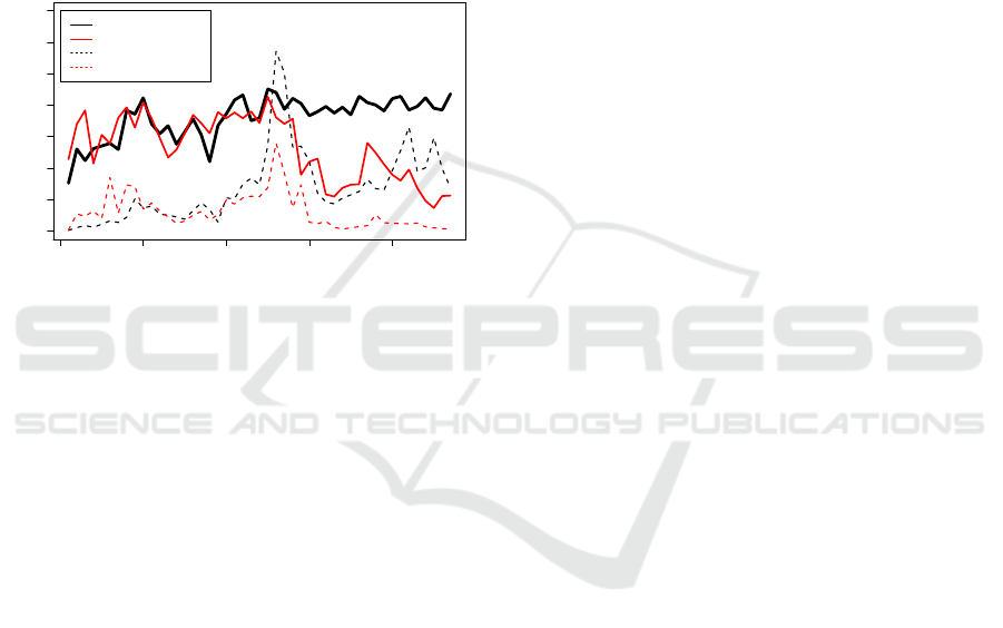
Max perform best. Additionally, we tested another
case where we set the probability to create a docu-
ment from f
1
5 times higher than f
2
. This causes
the number of co-occurrences for w
51
, w∗ to rise up
as well which is caused by the noise introduced by
f
Zip f
. The chance of sampling a word from the noise
in combination with w
51
is also higher when sam-
pling more often from f
1
according to formula 8. This
introduces more co-occurrences with a low signifi-
cance and the significance-based algorithms tend to
diminish the overall volatility (figure 7). For this ad-
ditional test case we only compared the target func-
tions triangle and sinus. Both respective factors use
the same amount of maximal changes for the time
stamps. In table 2 we show the mean distances be-
tween the volatility values and the expected target
function value. When working with real data (Vo-
cabsize >> 1000) this problem goes to the point,
where the resulting context volatility is inversely pro-
portional to the words frequency. For words with dif-
ferent frequency but similar context changes this re-
sults in different values for the context volatility. The
shape of two context volatility time series might be
similar but differs in the value range. When measur-
ing a global volatility among all T , 2 words of dif-
ferent frequency classes are not comparable in values
even though their contextual change would be com-
parable. Such being the case we cannot compare 2
words, which differ in frequency, considering their
context volatility in a reliant manner when using sig-
nificance based algorithms.
Table 2: Mean distances between the calculated volatility
and the target function at each point of time; the factor re-
flecting the triangle function was used 5 times more than the
one for sinus.
MinMax Sig
Triangle 0.13 0.27
Sinus 0.12 0.15
Comprising the evaluation, the MinMax-
algorithm is the most consistent method against
differences in term frequency and different types
of contextual change. Even though we draw our
conclusion based just on a synthetic dataset, we do
so knowing that the synthetic dataset was specially
designed to make the problems which arise when
working with real data measurable.
6 EXAMPLE ON REAL DATA
In this section we apply the MinMax-algorithm to
process 8156 British newspaper articles from January
1st until November 30th of 2016 which include the
words brexit and referendum.
2
The used language is
English, but the concept of context volatility is lan-
guage independent. The subject of interest for this
analysis of context volatility are keywords surround-
ing the “Brexit“ referendum in 2016. We split the
documents into sentences, removed stopwords and
used stemming. Furthermore we split the data set into
time slices of weeks. We used the dice coefficient
as significance-weight for the co-occurrences in sen-
tences. The MinMax-algorithm was applied using a
span of 3 weeks (h = 3).
0.0 0.1 0.2 0.3
0 10 20 30 40
context volatility
weeks
brexit
farage
cameron
may
referendum
Figure 3: Context volatility for the words brexit, cameron,
may and farage.
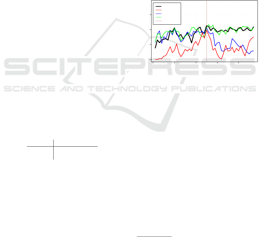
In figure 3 the measured context volatilities for the
words brexit, farage, cameron and may are shown.
The time of the referendum is included as dotted
slash. One can identify different ways of contex-
tual change for the words. For example, the context
for the word cameron reveals some high amount of
change, which suddenly drops right after the refer-
endum. This goes along with the announcement of
Camerons resignation after the referendum. There is
basically no new or altered information resulting in a
decrease of context volatility. In this sense, context
volatility seems also to track the currentness of infor-
mation in consecutive time stamps. In comparison to
that we can see an allover high value for may, which is
even a little bit higher after the referendum. Theresa
May, being the designated prime minister might ex-
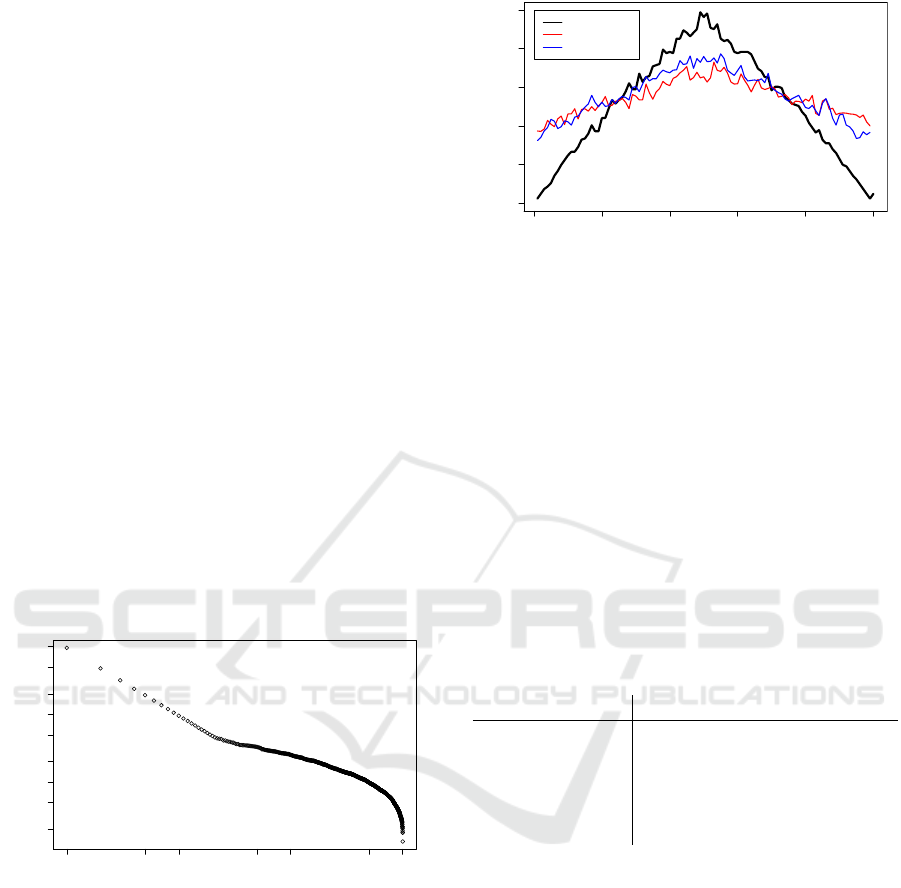
plain these results. In figure 4 the volatility values for
brexit and cameron are shown with their respective
frequencies. Although there is some correlation be-
tween volatility and frequency, it is obvious that there
are lots of phenomena in the volatility values, which
2
We used the Guardian API (http://open-
platform.theguardian.com/) to acquire the documents.
can’t be explained just by frequency. Especially for
the word brexit, we notice continuously a high volatil-
ity value irrespective of its frequency. In the time
immediately around the referendum the frequency of
both words have their highest peaks, which is caused
by the amount of articles released at that time span.
However, we measure almost the same amount of
contextual change for brexit already in February just
after Cameron announced the referendum, indicating
at that stage a high degree of public controversy. Us-
ing the MinMax-algorithm, we can compare a word’s
volatility with its frequency over time as well as 2
words that differ in frequency.
0.00 0.10 0.20 0.30
0 10 20 30 40
context volatility
weeks
brexit−cv
cameron−cv
brexit−frequency
cameron−frequency
Figure 4: Context volatility for the words brexit, cameron
and their frequencies.
7 CONCLUSION
In this work we presented an evaluation and prac-
tical application of the context volatility methodol-
ogy. We’ve shown a solution for evaluating con-
textual change measurements, especially the con-
text volatility measure, by creating a synthetic data
set, which can simulate various cases of contextual
change. Also, we introduced alternative algorithms,
which are superior to the baseline context volatility
algorithm, when facing problems on real diachronic
corpora (co-occurrence gaps). In the evaluation and
application the MinMax-algorithms shows its robust-
ness when competing with other methods by the abil-
ity to use the gap information directly and handle
the dynamics in the number of co-occurrences for a
word. With those improvements in the calculation of
context-volatility, we believe that the measure is able
to produce new results in various applications.
REFERENCES
Blei, D. M. and Lafferty, J. D. (2006). Dynamic topic mod-
els. In Proceedings of the 23rd international confer-
ence on Machine learning, pages 113–120.
Bordag, S. (2008). A comparison of co-occurrence and sim-
ilarity measures as simulations of context. In Com-
putational Linguistics and Intelligent Text Processing,
pages 52–63. Springer.
Fernndez-Silva, S., Freixa, J., and Cabr, M. T. (2011).
Picturing short-period diachronic phenomena in spe-
cialised corpora: A textual terminology description
of the dynamics of knowledge in space technologies.
Terminology, 17(1):134–156.
Hamilton, W. L., Leskovec, J., and Jurafsky, D. (2016). Di-
achronic word embeddings reveal statistical laws of
semantic change. arXiv preprint arXiv:1605.09096.
Heyer, G., Holz, F., and Teresniak, S. (2009). Change
of Topics over Time and Tracking Topics by Their
Change of Meaning. In KDIR ’09: Proc. of Int. Conf.
on Knowledge Discovery and Information Retrieval.
Heyer, G., Kantner, C., Niekler, A., Overbeck, M., and
Wiedemann, G. (2016). Modeling the dynamics of
domain specific terminology in diachronic corpora.
In TERM BASES AND LINGUISTIC LINKED OPEN
DATA, pages 75 – 90.
Heyer, G., Keim, D., Teresniak, S., and Oelke, D. (2011).
Interaktive explorative Suche in groen Dokumentbest-
nden. Datenbank-Spektrum, 11(3):195–206.
Holz, F. and Teresniak, S. (2010). Towards Automatic De-
tection and Tracking of Topic Change. In Computa-
tional Linguistics and Intelligent Text Processing, vol-
ume 6008, pages 327–339. Springer, Berlin, Heidel-
berg.
J
¨
ahnichen, P. (2016). Time Dynamic Topic Models.
J
¨
ahnichen, P., Oesterling, P., Liebmann, T., Heyer, G.,
Kuras, C., and Scheuermann, G. (2015). Exploratory
Search Through Interactive Visualization of Topic
Models. Digital Humanities Quarterly.
Jatowt, A. and Duh, K. (2014). A framework for analyzing
semantic change of words across time. In Proceed-
ings of the 14th ACM/IEEE-CS Joint Conference on
Digital Libraries, pages 229–238.
Jurish, B. (2015). DiaCollo: On the trail of diachronic col-
locations. In De Smedt, K., editor, CLARIN Annual
Conference 2015 (Wro\law, Poland, October 1517
2015), pages 28–31.
Kenter, T., Wevers, M., Huijnen, P., and de Rijke, M.
(2015). Ad hoc monitoring of vocabulary shifts over
time. In Proceedings of the 24th ACM International
on Conference on Information and Knowledge Man-
agement, CIKM ’15, pages 1191–1200.
Kim, Y., Chiu, Y.-I., Hanaki, K., Hegde, D., and Petrov, S.
(2014). Temporal analysis of language through neu-
ral language models. In Proceedings of the ACL 2014
Workshop on Language Technologies and Computa-
tional Social Science, pages 61–65.
Michel, J.-B., Shen, Y. K., Aiden, A. P., Veres, A.,
Gray, M. K., The Google Books Team, Pickett, J. P.,
Hoiberg, D., Clancy, D., Norvig, P., Orwant, J.,
Pinker, S., Nowak, M. A., and Aiden, E. L. (2011).
Quantitative Analysis of Culture Using Millions of
Digitized Books. Science, 331(6014):176–182.
Mitra, S., Mitra, R., Riedl, M., Biemann, C., Mukherjee, A.,
and Goyal, P. (2014). That’s sick dude!: Automatic
identification of word sense change across different
timescales. In Proceedings of the 52nd Annual Meet-
ing of the Association for Computational Linguistics
(Volume 1: Long Papers), pages 1020–1029, Balti-
more, Maryland. Association for Computational Lin-
guistics.
Picton, A. (2011). A proposed method for analysing the
dynamics of cognition through term variation. Termi-
nology, 17(1):49–74.
Rohrdantz, C., Hautli, A., Mayer, T., Butt, M., Keim, D. A.,
and Plank, F. (2011). Towards Tracking Semantic
Change by Visual Analytics. In Proceedings of the
49th Annual Meeting of the ACL: Human Language
Technologies: Short Papers - Volume 2, pages 305–
310.
Rohrdantz, C., Niekler, A., Hautli, A., Butt, M., and Keim,
D. A. (2012). Lexical Semantics and Distribution of
Suffixes: A Visual Analysis. In Proceedings of the
EACL 2012 Joint Workshop of LINGVIS & UNCLH,
pages 7–15.
Simpson, J. A., Weiner, E. S. C., and Oxford University
Press, editors (1989). The Oxford English dictionary.
Clarendon Press; Oxford University Press, Oxford:
Oxford; New York, 2nd ed edition.
Taylor, S. J. (2007). Introduction to Asset Price Dynamics,
Volatility, and Prediction. In Asset Price Dynamics,
Volatility, and Prediction. Princeton University Press.
Wijaya, D. T. and Yeniterzi, R. (2011). Understanding Se-
mantic Change of Words over Centuries. In Proceed-
ings of the 2011 International Workshop on DETecting
and Exploiting Cultural diversiTy on the Social Web,
DETECT ’11, pages 35–40, New York, NY, USA.
ACM.
Zhang, J., Song, Y., Zhang, C., and Liu, S. (2010). Evo-
lutionary hierarchical dirichlet processes for multiple
correlated time-varying corpora. In Proceedings of
the 16th ACM SIGKDD international conference on
Knowledge discovery and data mining, pages 1079–
1088.
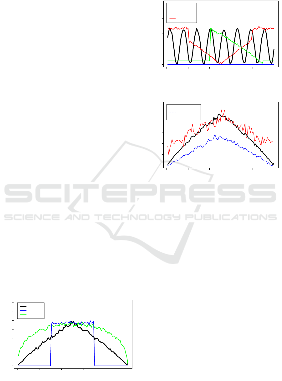
APPENDIX
0 10 20 30 40 50 60 70
0 20 40 60 80 100
number of changes
time
triangle
hat
halfcircle
Figure 5: Three target functions showing the amount of
changes in the function factors in dependence to the time
0 20 40 60 80
0 20 40 60 80 100
number of changes
time
sinus
no_change
slide
canyon
Figure 6: Other 4 target functions showing the amount of
changes in the function factors in dependence to the time
0.0 0.2 0.4 0.6 0.8 1.0
0 20 40 60 80 100
context volatility
time
target−function
Sig
MinMax
Figure 7: Triangle target function and the calculated volatil-
ities using MinMax and Sig with high frequence for refer-
ence word
