Methods for Hemodynamic Parameters Measurement
using the Laser Speckle Effect in Macrocirculation
Pedro G. Vaz
1,2
, Anne Humeau-Heurtier
2
, Edite Figueiras
3
and Jo
˜
ao Cardoso
1
1
LIBPhys-UC, Department of Physics, University of Coimbra
Rua Larda, Coimbra 3004-516, Portugal
2
University of Angers, LARIS - Laboratoire Angevin de Recherche en Ing
´
enierie des Syst
`
emes,
62 avenue Notre-Dame du Lac, 49000 Angers, France
3
International Iberian Nanotechnology Laboratory, Avenida Mestre Jos
´
e Veiga, s/n,
4715-330, Braga, Portugal
Abstract. This chapter present a set of studies that have been developed with the
goal of probing the possibilities of using laser speckle effect as a tool to extract
macrocirculatory hemodynamic parameters. Within this project, a laser speckle
prototype has been constructed and three bench experiment have been designed.
The first bench experiment consists on using multi-wavelength light sources to
extract the vibration frequency of a phantom and heart rate of several subjects.
The second experiment consists on the extraction of the pulse pressure waveform
using the same instrumentation and processing algorithms as the ones used on
microcirculation laser speckle imaging. Finally, a pilot study was also designed
in order to use laser speckle for 2D image segmentation. The obtained results re-
vealed that laser speckle has the capability to extract macrocirculatory hemodyn-
amic parameters and that this feature can be included in commercially available
devices. In this sense, the ability to extract macrocirculatory and microcirculatory
parameters could lead to interesting commercial advantages.
1 Introduction
Laser speckle has been considered as a side effect of using polarized light since the first
laser based applications. Speckle can be defined as the visualization of a dark and bright
dot pattern resulting from the interference of the coherent light when it is reflected by a
rough surface or liquid media containing scatterers. This effect limits the contrast, spa-
tial resolution and signal-to-noise ratio (SNR) of laser based applications such as optical
coherence tomography (OCT) [1]. However, for a long time that speckle imaging has
been used as source of important information. It has been used as static material cha-
racterization technique because it contains information on the surface morphological
properties [2] and also on dynamic material strain characterization [3].
The first reference of a biomedical application of laser speckle imaging (LSI) can
be found in the pioneer work of Fercher and Briers (1981) [4] where speckle was used
to analyze the retina blood flow, a typical application for microcirculation assessment.
Since then, LSI has been studied and improved by many researchers that believe this
28
Vaz P., Cardoso J., Humeau-Heurtier A. and Cardoso J.
Methods for Hemodynamic Parameters Measurement using the Laser Speckle Effect in Macrocirculation.
DOI: 10.5220/0007902200280045
In European Project Space on Networks, Systems and Technologies (EPS Porto 2017 2017), pages 28-45
ISBN: 978-989-758-310-0
Copyright
c
 2017 by SCITEPRESS – Science and Technology Publications, Lda. All rights reserved

technique is able to provide important physiological informations with benefits over the
existing methods. Most works related with LSI still focus on the assessment of blood
flow inside small arteries, either in the development of new LSI instrumentation or
improving the existing mathematical theories. Most LSI scientific research relates with
the two major technique issues, which are the improvement of its assessment depth and
the determination of quantitative blood flow values.
The following paragraphs summarize some reference works on LSI during the past
two decades in order to give an overview of current situation. David Boas and An-
drew Dunn have developed many important works on LSI, one in particular, Boas and
Dunn (2010) [5], presents an important explanation of the laser speckle imaging phy-
sics. Parthasarathy et al. [6] proposed an accurate LSI technique based on the acqui-
sition of the speckle patterns using multiple exposure times. This same technique has
also been explored by Kazmi et al. [7] several years later. Ramirez-San-Juan et al. [8]
have studied the influence of static scatterers in two LSI image analysis methods, the
spatial and temporal laser speckle contrast. The effect of static scatterers is an impor-
tant research line also explored by Zahkarov et al. [9] by developing new theoretical
concepts to correct this effect. Varma et al. [10] and Huang et al. [11] presented works
on laser speckle tomography, which is a recently developed LSI variation that impro-
ves the assessment depth of speckle imaging. Some LSI methodological reviews have
been presented by Senarathna et al. [12], Briers et al. [13] and Vaz et al. [14]. Finally,
the latest developments on laser speckle research ranging from theoretical analysis to
practical application can be found in [15–18].
Laser speckle imaging has been strongly focused on microcirculatory applications
but it can also be used as a tool for macrocirculatory assessment. This chapter starts by
introducing some simple laser speckle imaging theoretical (section 2) concepts neces-
sary for the comprehension of the experiments. Next, an overview of physiological con-
cepts (section 3) related with the macrocirculation physiology is presented. After that,
the experimental tests, developed for proof of concept, will be presented (section 4) and
their results discussed (section 5). Finally, the conclusions are presented in section 6.
2 Laser Speckle Imaging
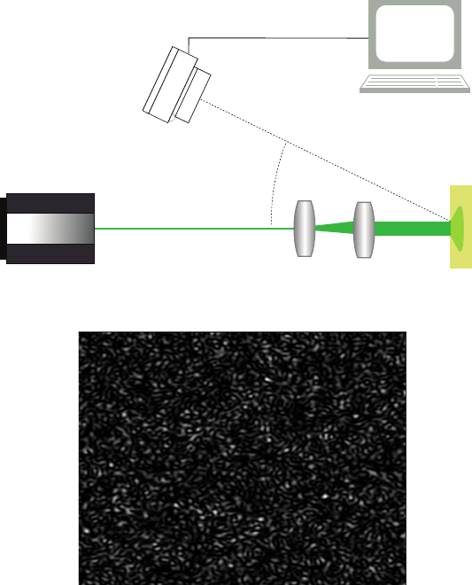
2.1 Instrumentation Set-up
The LSI technique is often based on the illumination of a sample using a coherent
light source, as a laser, and the detection of the reflected light using a video camera.
In order to analyzed samples with large areas, a beam expander needs to be coupled
onto the laser beam. To these two critical elements, adds up a signal processing and
control module which can be a standard PC or dedicated hardware. This module is
responsible for the image collection, from the video camera, and is responsible for
digitally process them in order to extract valuable information. Figure 1 represent a
standard LSI instrumentation.
Figure 2 shows an example of a synthesized laser speckle pattern of a static target
with 800 × 600 pixels. This figure has been synthesized using the algorithm described
in [19]. The dark and bright spots are clearly visible in this figure and, since it results
from a static target, they are very sharp.
29
Methods for Hemodynamic Parameters Measurement using the Laser Speckle Effect in Macrocirculation
29

Laser
Video
Camera
Target
Beam expander
Control and acquisition module
Fig. 1. Typical LSI instrumentation set-up.
100 200 300 400 500 600 700 800
100
200
300
400
500
600
Fig. 2. Synthetic laser speckle pattern of a static target.
When the imaged target is moving or contains dynamic scatters, the resultant speckle
pattern changes. These type of patterns are called dynamic speckle patterns and they
are the ones that we are interested in when assessing macrocirculatory parameters. In
practical applications, the video camera used to image the pattern has a finite exposure
time. During this time, the camera integrates all the different reflected speckle patterns.
The integration of these patterns results in a blurred final image. The blurring degree
contains information of how much the speckle pattern changed during the integration
time.
2.2 Mathematical Description
A simple way to quantify the blurring degree of a speckle image is by computing its
contrast. Speckle contrast (K) is usually defined as the quotient between the image
standard deviation and the mean intensity [20]:
30
EPS Porto 2017 2017 - European Project Space on Networks, Systems and Technologies
30

K =
σ
s
hIi
=
q

(I − hIi)
2

hIi
, (1)
where σ
s
corresponds to the standard deviation and hIi corresponds to the pattern mean
intensity. It has been demonstrated that, giving the speckle statistical properties under
real conditions, the value of speckle contrast is bounded by the interval [21]:
0 ≤ K ≤ 1 . (2)
A contrast value of 1 implies a fully developed speckle pattern, which means that
the speckles in the pattern are temporally correlated. On contrary, a contrast value of 0
corresponds to a blurred speckle pattern where the speckles changed during the integra-
tion time, i.e. are temporally decorrelated.
In practical applications, the contrast value of a speckle pattern never reaches the
unitary value. The lack of perfect polarization, system imperfections, stability of light
source and the speckle averaging on the image detector results in the decrease of the
maximum speckle contrast that can be measured [22].
Apart from speckle contrast, a different metric can be used to quantify the speckle
pattern changes between consecutive frames. This metric is the two dimensional corre-
lation coefficient and can be defined as:
r =
P
x
P
y
(A
xy
−
¯
A)(B
xy
−
¯
B)
q
(
P
x
P
y
(A
xy
−
¯
A)
2
)(
P
x
P
y
(B
xy
−
¯
B)
2
)
, (3)
where A and B are two consecutive images,
¯
A and
¯
B is the average pixel intensity of
each image and the indexes x and y the pixel position in the image.
2.3 Experimental Considerations
When developing laser speckle imaging devices and experiments, an important con-
sideration on the speckle size must be taken into account. In order to prevent spatial
aliasing, the speckle size should be, at least, two times the pixels size (2 speckles/pixel)
in both x and y directions. A following theoretical equation can be used to compute the
speckle size of the system [23]:
d
min
≈ 1.2(1 + M)λf/# , (4)
where d
min
corresponds to the minimum speckle diameter, λ is the light wavelengths,
M is the imaging system magnification, and f/# is the imaging lens f-number. Consi-
dering this equation, the speckle size can be controlled by changing the imaging system
aperture. An empirical way to determine the speckle size is to compute the 2D power
spectral density (PSD) of a static speckle pattern and apply the following equation [24]:
d
min
= 2
l
P SD
d
energy
, (5)
where l
P SD
is the power spectral density width, in pixels and d
energy
is the diameter
of the energy band.
31
Methods for Hemodynamic Parameters Measurement using the Laser Speckle Effect in Macrocirculation
31

3 Macrocirculation Physiology
Regarding the macrocirculation, some of the most important physiological parameters
can be highly summarized as the blood pressures (systolic and diastolic), the pulse wave
velocity, and the profile of the pulse waveform. In this work we have been focused on
extracting the pulse pressure waveform because it is the parameter that can be measured
using laser speckle optical methods.
The pulse pressure waveform is not constant along all the arterial tree. Both its shape
and intensity changes, starting with a strong pulsation component at the major arteries
and ending in a static pressure value at the capillaries. The valuable information on the
pulse waveform is encoded in its shape so it is mandatory to assess major arteries. The
aorta should be the right choice because it is closer to the heart and produces higher
SNR but, in order to assess it, an invasive probe will be necessary. Since we are interest
in non-invasive instrumentation, arteries like the carotid or radial must be used because
they are superficial and still contain valuable information.
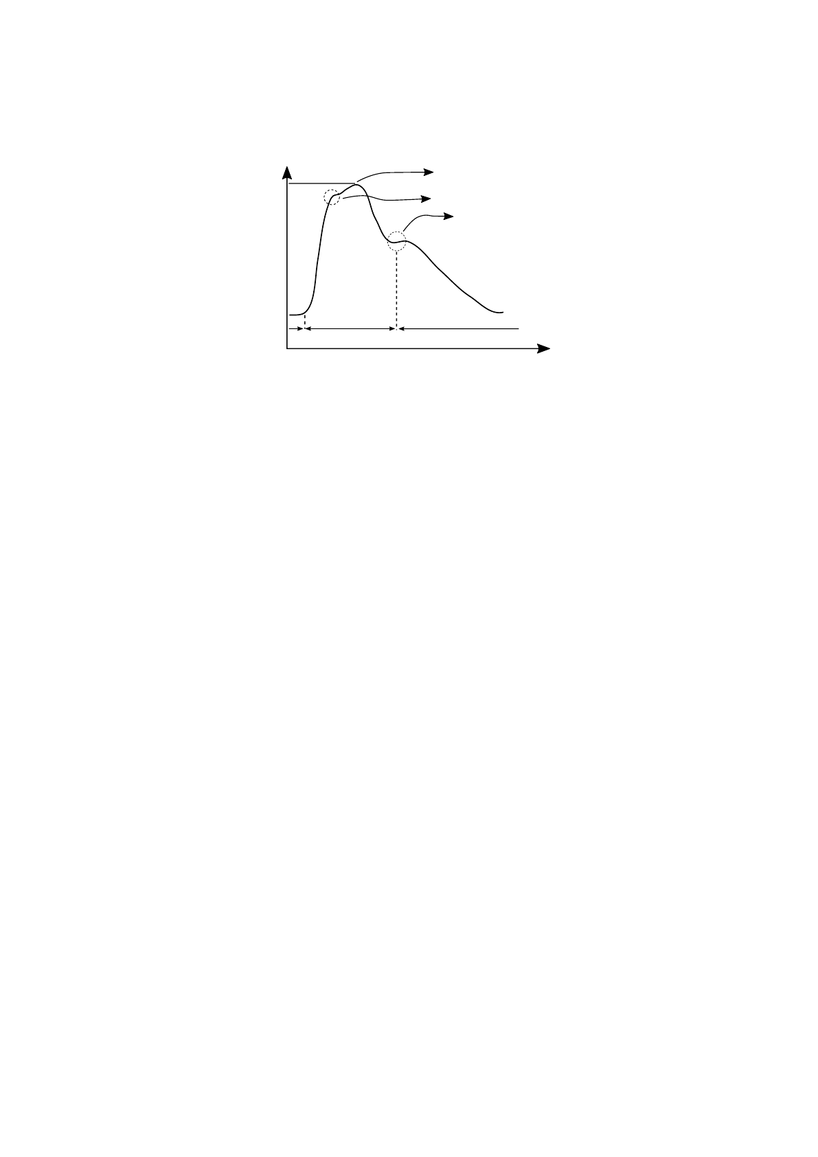
The aortic pulse pressure profile is detailed in figure 3. The systolic peak corre-
sponds to the highest pressure value, the dicrotic notch is induced by the aortic valve
closure and, the diastolic pressure corresponds to the minimum pressure value [25].
This figure corresponds to a typical profile from an unhealthy subject because the re-
flected wave, also represented in the figure, appears before the systolic peak, resulting
in an increase of the maximum pressure [26].
By identifying these feature points (systolic peak, reflected wave, dicrotic notch)
many important parameters can be extracted even when the pressure waveform is not
amplitude calibrated. This method, called pulse waveform analysis (PWA), can deter-
mine many indices of the cardiovascular function like the Augmentation index (AIx),
Ejection Time Index (ETI), Subendocardial Viability Ratio (SEVR %), maximum rate
of pressure change (dP/dt
max
) and area under the curve (AUC) [26].
Apart from these parameters that can be extracted by PWA, the pulse waveform
velocity (PWV) can only be computed by assessing two pulse pressure waveform in
different sites. This parameters corresponds to the propagation velocity of the pulse
waveform and can be determined by computing the time delay between the detection of
the same pulse waveform in two sensors separated by a known distance.
In this work, the computations of these parameters were not performed since our
aim it to focus on instrumentation development and proof of concept. However, it is im-
portant to understand why this field has clinical relevance and what type of information
can be extracted from this data.
4 Experimental Methods
Three different tests have been developed during this work in order to test the ability of
LSI to extract the pulse pressure waveform. In the first test, three different light wave-
lengths have been tested in order to select the better one [28]. In the second experiment,
only the best wavelength was used and the group of volunteers has been extended [29].
The last experiment consists in a pilot study that used LSI in order to segment a target
with longitudinal motion [30]
32
EPS Porto 2017 2017 - European Project Space on Networks, Systems and Technologies
32

Pressure
Time
DP
SP
Dichrotic Notch
Systolic Peak
Refected wave
Aortic valve
opened
Aortic valve
closed
Fig. 3. Aortic pressure waveform. SP - Systolic pressure. DP - Diastolic pressure [27].
4.1 Multiwavelengths Study
The experimental set-up described in subsection 2.1 was used to study which wave-
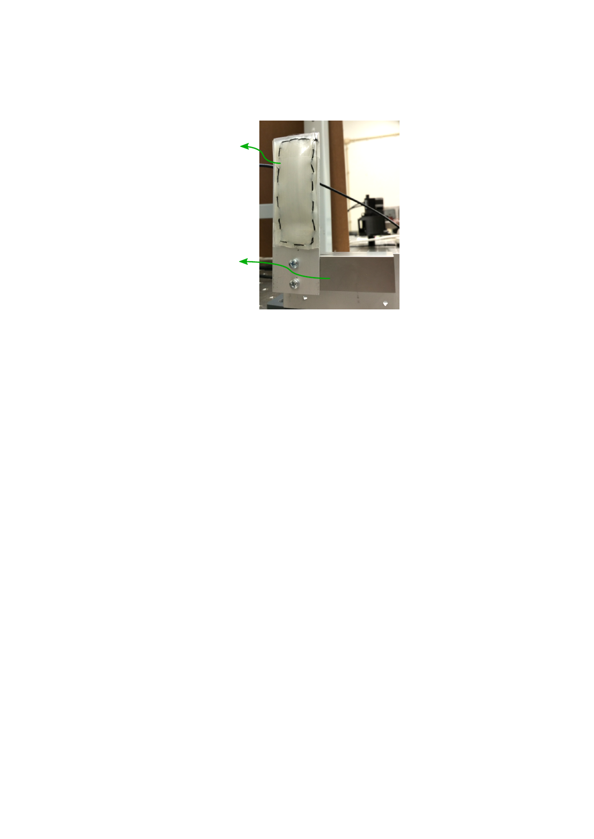
length is better to extract the pulse waveform. The target on this set-up was replaced
by a phantom that tries to mimic the radial artery motion, which is the primary site for
the application of this method. The phantom was built by stacking 4 white translucent
silicone membranes with a total thickness of 2 mm and a size of 30 mm × 60 mm (W
× H). It has been attached to a controlled piezoelectric actuator that reproduced sinus-
oidal movements with different amplitudes and frequencies. The phantom is depicted
in figure 4.
The phantom was actuated with amplitudes ranging from 2 peak-to-peak voltages
(V
pp
) to 8 V
pp
and frequencies ranging from 1/5 Hz to 1 Hz. These combinations of
parameters lead to phantom maximum displacements of 0.75 mm and velocities up to
2.35 mm/s.
Three different light sources have been used in this experiment: a green laser diode
(L
532
), Thorlabs ref. CPS532, with a wavelengths of 532 nm, with optical power of
4.5 mW and with an output circular beam; a red laser diode (L
635
), Coherent inc. ref.
VHK, with a wavelength of 635 nm, with an optical power of 4.9 mW and, with a
circular beam; and a near infra-red laser diode (L
850
), with a wavelength of 850 nm,
with an optical power of 3mW, and with a focusable elliptical beam.
Finally, a monochrome video camera (Pixelink - B741U), attached to a fixed focal
lengths lens (50 mm), was used to image the speckle patterns. By using equation (4),
the optimal f-number to ensure a correct sampling (4 pixels/speckle) was computed and
corresponds to f/16. The camera has been set-up to a resolution of 1280 × 1024 pixels,
with an exposure time of 15 ms and with a frame rate of 15 frames per second (fps).
The acquisition time has been 7 seconds for all the acquisitions.
The speckle patterns have been processed using the two dimensional correlation
coefficient detailed in equation (3). This processing technique only requires the com-
putation of one coefficient for each image pair. In order to easy visualize the data, the
correlation coefficient was normalized between 0 and 1 (r
0
) and inverter (1 − r
0
).
33
Methods for Hemodynamic Parameters Measurement using the Laser Speckle Effect in Macrocirculation
33

Skin-like
Phantom
Piezo-electric
Actuator
Fig. 4. Photography of the skin-like phantom connected to the piezo-electric actuator [27].
After the bench experiment, a small in vivo study was also performed by assessment
the radial artery of two healthy volunteers. The volunteers have provided written infor-
med consent prior to participation. Due to the complexity of the biological systems, the
video cameras frame rate was increased to 50 fps and the image resolution decreased
to 320 × 240 pixels due to the hardware limitation. For each subject, 9 acquisitions
have been performed, three for each laser source, after a 5 minute rest. Each acquisition
last for 10 seconds. A photopletismography (PPG) probe was used to assess the pulse
waveform but due to synchronization problems both signals could not be visualized at
the same time.
4.2 In vivo Study
The in vivo study has been developed in order to test the better laser light source in
a more intensity experiment and using the same processing methods used for LSI mi-
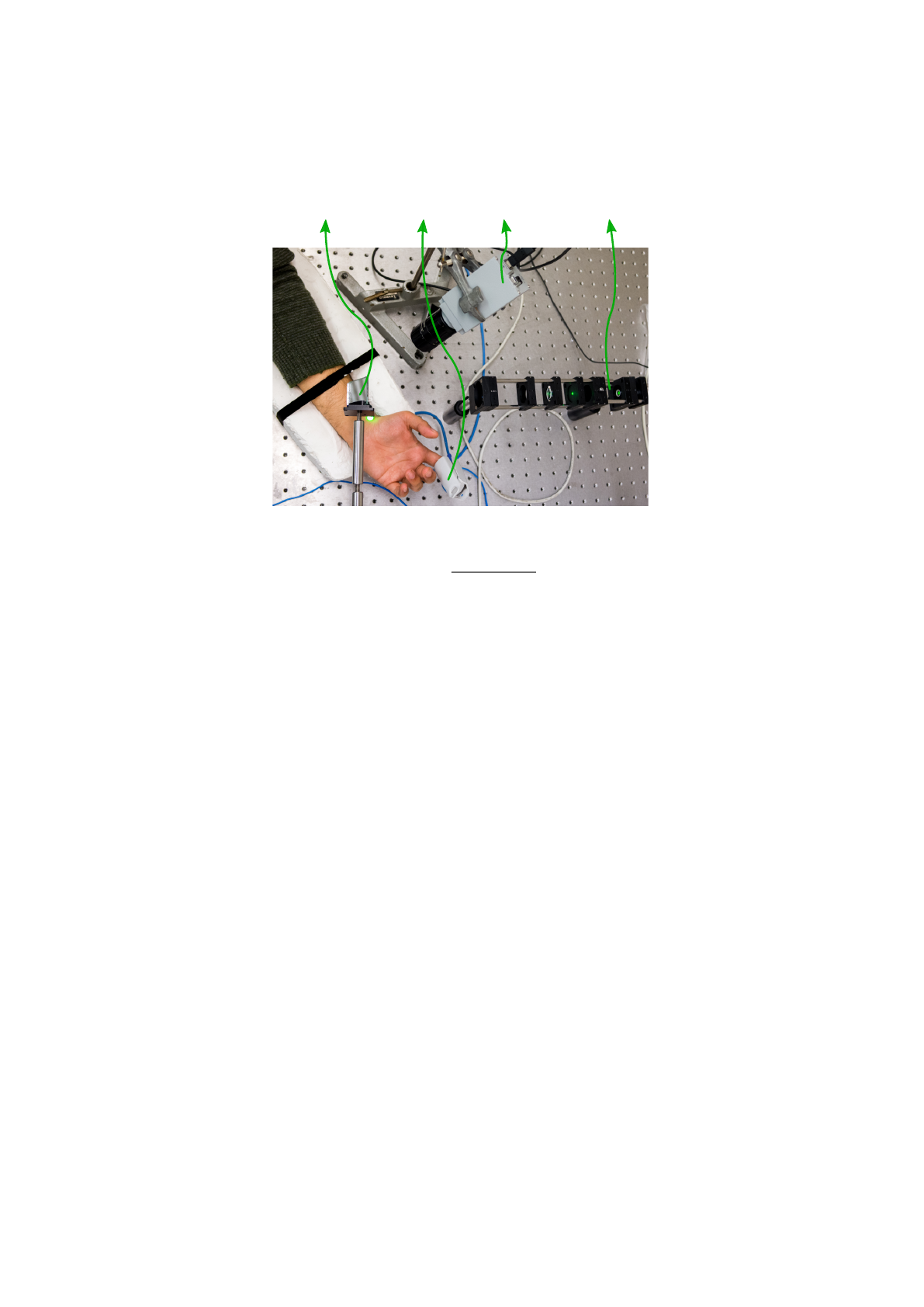
crocirculation assessment. Figure 5 shows the experimental setup including the video
camera, the beam expander, the subject arm and the PPG probe. In this study, the PPG
signal (P P G(t)) has been synchronized with the LSI signal which has allowed a better
comparison between both. This test was performed in 10 subjects with 3 acquisitions
per subject. Each acquisition lasts 10 seconds.
Unlike the previous experiment, in this study, the LSI data was processed using the
speckle contrast method (equation (1)). One contrast value for each LSI image has been
computed. Again, the contrast values (K(t)) have been inverted (K’(t)) due to the inverse
relation between speckle contrast and motion, and normalized between -1 and 1. The
signal obtained with the PPG was also normalized in order to facilitate the comparison.
For each acquisition, the heart rate (HR) of the subject was computed by using the
fast Fourier transform (FFT) algorithm and identifying the predominant frequency. The
data similarity has been assessed by computing the spectral coherence between both
signals by using the magnitude-squared coherence function:
34
EPS Porto 2017 2017 - European Project Space on Networks, Systems and Technologies
34

Mirror
PPG
probe
Video
camera
Ilumination
system
Fig. 5. In vivo acquisition scheme for laser speckle imaging and PPG recording.
C
KP
(f) =
|P
KP
(f)|
2
P
K
(f)P
P
(f)
, (6)
where P
KP
(f) is the cross-spectral power between K(t) and P P G(t), while P
K
(f)
and P
P
(f) are the PSD of K(t) and P P G(t), respectively. A similarity index (SI)
(equation (7)) was then defined as the integral of the magnitude-squared coherence
function between 0 and 10 Hz because this band contains the relevant information:
SI =
Z
10
0
C
KP
(f)df . (7)
4.3 Image Segmentation Study
The last study has been developed in order to explore the possibility of LSI to identify
and segment targets with longitudinal motion without any stereoscopic data or other
types of sensors. This type of movement is difficult to identify because it occurs on the
imaging axis but speckle methods can be useful in these situations. Moreover, this pilot
study aims at segment a target with specular reflection similar to skin and soft tissues.
For this test, the apparatus described in figure 1 was modified in order to include
a second target. The new target, identical to the first one, has been placed next to the
original one. A small gap of 3 mm was left between the targets. The main idea behind
this new phantom was to have two identical independent membranes, one connected
to the piezoelectric actuator and other completely static. The moving membrane was
actuated with a sinusoidal movement with frequencies of 1, 1/2, 1/3 and 1/5 Hz and
amplitudes of 1, 2, 4 and 6 V
pp
.
35
Methods for Hemodynamic Parameters Measurement using the Laser Speckle Effect in Macrocirculation
35

In this test, the used light source was the L
635
with a video camera resolution of
1280 × 1024 pixels and an exposure time of 15 ms. The speckle patterns have been
processed using a temporal backward difference in order to enhance the changes bet-
ween consecutive patterns. The result was then normalized between 0 and 255 and can
be defined as:
∆I(x, y, t) =
I(x, y, t) − I(x, y, t − 1) + 255
2
, (8)
where ∆I(x, y, t) is the derivative of the pixel with the position (x, y) and time t.
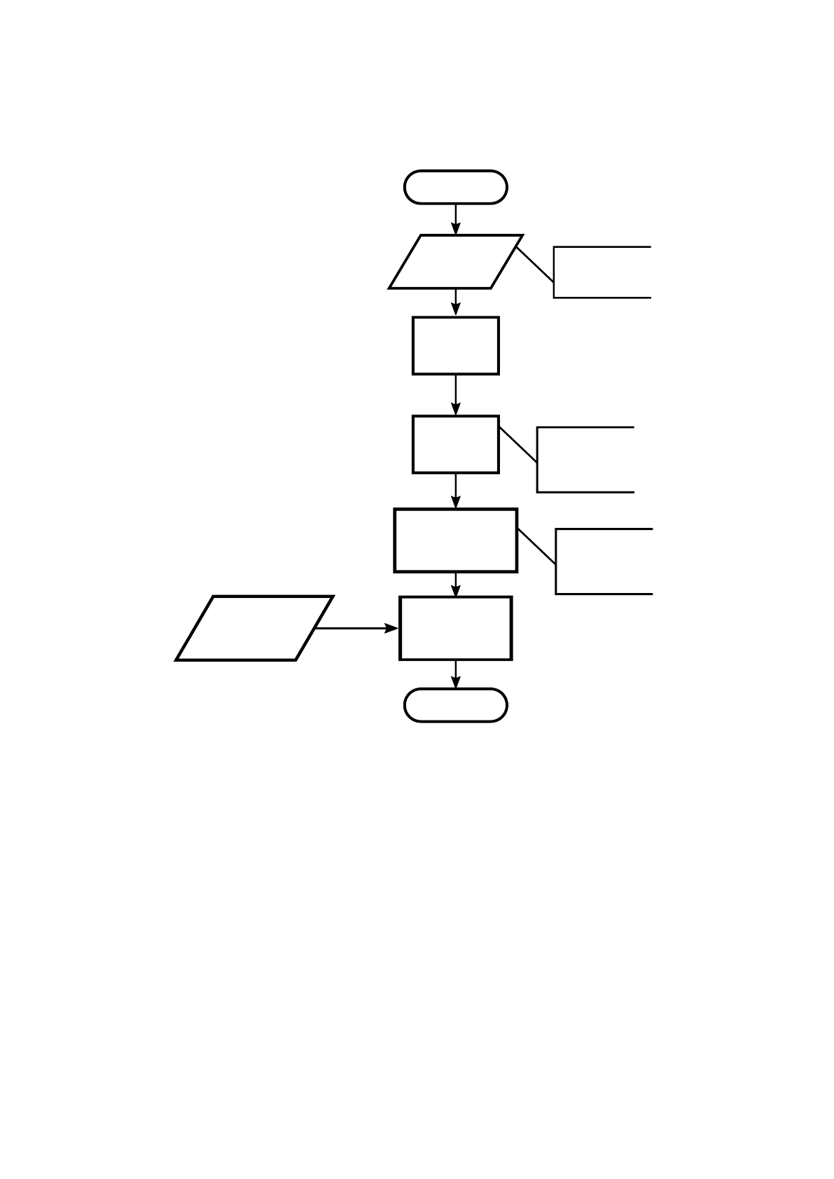
After this step, the segmentation was performed by computing the regional entropy
(RE) of the difference image (∆I). The regional entropy is an algorithm that computes
the entropy of small regions within the complete image with full overlap. In this algo-
rithm, this small regions have been tested for 4 different sizes, 3×3, 9×9, 27×27, and
81×81. For each region, the RE can be computed as:
RE = −
255
X
bin=0
P
bin
× log
2
(P
bin
) , (9)
where P
bin
is the probability of the occurrence of a pixel with value bin in the region.
The bin values range from 0 to 255.
The produced two dimensional entropy map is finally segmented by applying a
threshold. Pixels with entropy above this value have been classified as moving (1) and
pixels with entropy below this value have been classified as non-moving (0). The flow-
chart of this algorithm is presented in figure 6.
The most suitable region size has been determined by computing the sensitivity (SE)
and specificity (SP) for thresholds between 0 and 6 (the maximum value of entropy
computed in this experiment) with steps of 0.05. With these data, a receiver operatic
characteristic (ROC) curve has been plotted and its area under the curve (AUC) deter-
mined. The region with higher values of AUC has been considered as the most suitable
one.
A data-set of 12 entropy maps, containing membrane velocities from 0 to 1763
µms
−1
, was used to determine which threshold will lead to better results. This data-
set was selected in order to fully cover the range of membrane velocities presented in
this experiment. The best threshold corresponds to the one that maximizes the mean
accuracy (AC) of this training data-set.
Finally, the best region size and threshold have been applied to a test data-set com-
posed of 5 videos with different parameters (1 Hz-1V
pp
, 1 Hz-4V
pp
, 1/2 Hz-6V
pp
, 1/3
Hz-4V
pp
, and 1/5 Hz-1V
pp
). For each video, the AC, positive and negative predictive ra-
tios (PPV and NPV), and Matthews correlation coefficient (MCC) have been computed
[30].
5 Experimental Results
This section presents the results of the experiments described in section 4.
36
EPS Porto 2017 2017 - European Project Space on Networks, Systems and Technologies
36

Start
Get speckle data
Temporal
Derivative
Regional
entropy
Binarization
based on threshold
Manually segmented
mask
End
1280 x 1024
15 fps
Skin-like phantom
Optimal threshold
determined using
traning data-set
Optimal region size
determined using
ROC curve
Determination of
performance
parameters
Fig. 6. Flowchart of the method used to segment the moving skin-like phantoms.
5.1 Multiwavelengths Study
The raw speckle data have been processed and compared with the electrical signal app-
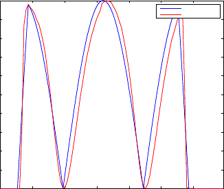
lied to the phantom. The figure 7 represents an example of a reconstruction of the velo-
city profile based on the computation of the speckle correlation coefficient. The blue
line corresponds to the velocity profile computed from the piezoelectric stimulation
signal. The red line corresponds to the inverse of the correlation coefficient normalized
between 0 and 1. Both profiles are very similar which demonstrates the ability of LSI
to extract the vibration profile of a skin-like phantom.
37
Methods for Hemodynamic Parameters Measurement using the Laser Speckle Effect in Macrocirculation
37

0 1 2 3 4 5 6
0
0.1
0.2
0.3
0.4
0.5
0.6
0.7
0.8
0.9
1
Velocity profile
Time (s)
Amplitude (A.U.)
Real
Estimated
Fig. 7. Plot of 1 − r
0
along time (red line) and absolute velocity of the phantom (blue line) of the
movement with amplitude of 2 V
pp
and 5 seconds of period.
The numerical result for all the movement parameters and lasers sources are presen-
ted in table 1. This values corresponds to the root mean square error (RMS) between the
real profile and the extracted profile. By analyzing the results for L
532
we can see that
larger periods are reconstructed with lower errors. This can be explained because lower
periods corresponds to higher membrane velocities and, due to the hardware limitations
on the frame rate (15 fps), faster movements are not acquired in good conditions. For
the case of L
635
light source, the errors decrease for movements with large periods and
small displacements. The explanation for this effect is the same as before. Finally, the
L
850
light source does not follow the other two cases because movements with higher
amplitudes present lower errors.
The overall errors for the three cases are close to each other with mean errors of
13.8%, 19.6% and 15.8% for L
532
, L
635
and L
850
respectively. However, it can be con-
cluded that the three laser sources have been able to reproduce the membrane velocity
profile with good results. Having said that, all the sources have been used in the in vivo
experiment.
The in vivo test lead to a different conclusion. First, all the laser sources presented
much lower SNR compared with the bench experiments. Moreover, the L
850
was unable
to record the pulse waveform of the two subjects. This occurred due to differences in
the optical properties of the skin-like phantom and the real tissue. In the human tissue,
the penetration and dispersion of the infra-red light is higher than in the phantom.
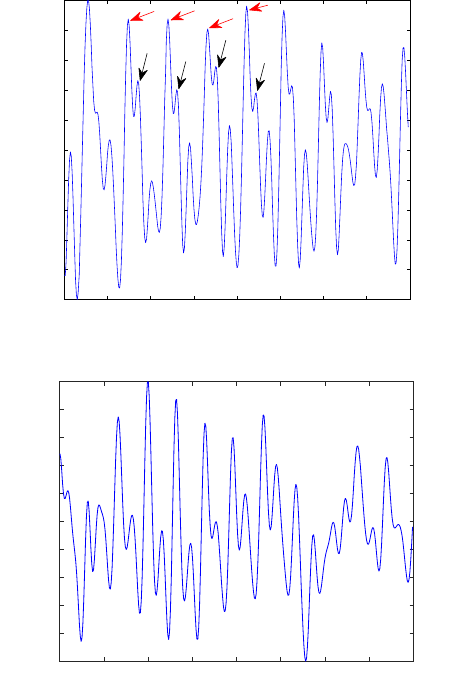
Figure 8 presents an example of two pulse waveforms extracted from L
532
(a) and
L
635
(b). The periodic nature of the pulse waveform is clearly identified in both figures.
The predominant oscillation frequency corresponds to the subject heart rate. In figure
8-(a) some pulse waveform features, like the systolic peak and dicrotic notch can also
be identified.
The numerical results of the HR determination are presented in table 2. The acquisi-
tion number S3 has been corrupted with motion artifacts which explains the large error
between the subject HR and speckle HR. The variable g 
rms
represents the global error
of each light source computed by the root mean square (rms) method. If the acquisition
38
EPS Porto 2017 2017 - European Project Space on Networks, Systems and Technologies
38

Table 1. Results of the RMS error of the velocity profile reconstruction with L
532
, L
635
and L
850
data. Values are presented in percentage.
Amplitude (V
pp
)
Period (s) 2 4 8
L
532
1 20.68 11.87 19.31
2 18.63 15.08 12.68
3 15.55 9.92 9.52
5 12.22 9.45 10.21
L
635
1 17.38 18.96 19.58
2 20.83 21.68 24.91
3 12.54 20.66 25.11
5 10.31 16.78 26.64
L
850
1 16.27 14.78 13.26
2 16.11 12.19 13.83
3 20.42 13.97 9.02
5 21.62 22.64 14.89
Table 2. Results of heart rate (HR) estimation with in vivo conditions. The values in the table are
expressed in beats per minute (bpm). * Data-set tainted by artifacts.
Data set S1 S2 S3* S4 S5 S6 g 
rms
L
532
Subject HR 62.3 62.3 64.1 65.9 67.8 67.8
Speckle HR 61.4 62.4 69.6 65.7 67.6 67.2 0.50 (2.28)
Data set S7 S8 S9 S10 S11 S12 g 
rms
L
635
Effective HR 64.1 65.9 67.7 82.4 89.7 60.4
Speckle HR 66.4 66.0 68.7 82.4 88.6 59.6 1.15
S3 is excluded from the analysis, the g 
rms
for the L
532
is much lower then the global
error of the L
635
, 0.5 bpm compared with 1.15 bpm.
These results in addition to the better graphical representation of figure 8 leads to the
conclusion that L
532
is the one that can extract the pulse waveform with higher SNR.
The lower tissue penetration of L
532
can explain why this was the wavelengths with
better results. For that reason, this light source was used in the second, more intensity,
in vivo study.
5.2 In vivo Study
In the second study, the speckle contrast was used as processing method in order to
match the signal processing technique already used by LSI commercial devices. Figure
9 presents an example of two speckle images captured at different cardiac cycle stages.
The speckle pattern of the stage when the artery is moving appears more blurred than
the speckle pattern when the artery is stopped, resulting in a contrast decrease of figure
9(a).
An example of the contrast values and the PPG data is shown on figure 10. The
profile of both signals is very similar and the identification of the feature points can be
done in the speckle contrast signal. This indicates good compatibility between the two
methods. The morphological differences between these signals are expected because
39
Methods for Hemodynamic Parameters Measurement using the Laser Speckle Effect in Macrocirculation
39

2 3 4 5 6 7 8 9 10
−1
−0.8
−0.6
−0.4
−0.2
0
0.2
0.4
0.6
0.8
1
In vivo correlation algorithm output
Time (s)
Amplitude (A. U.)
(a) L
532
Time (s)
2 3 4 5 6 7 8 9 10
Amplitude (A. U.)
-1
-0.8
-0.6
-0.4
-0.2
0
0.2
0.4
0.6
0.8
1
In vivo correlation algorithm output
(b) L
635
Fig. 8. Output signal of the correlation algorithm to the in vivo test S4 (a) and S10 (b). Red arrows
show the probable systolic peak and black arrows show the probable dicrotic notch.
they have been acquired in different sites (radial artery vs finger tip) which corresponds
to different locations on the arterial tree.
The HR identified by the PPG signal was considered as the correct one because pho-
topletismography is a well established technique. The heart rates detected in this study
range from 55 to 84 bpm with a mean value of 67 bpm corresponding to a normal rest
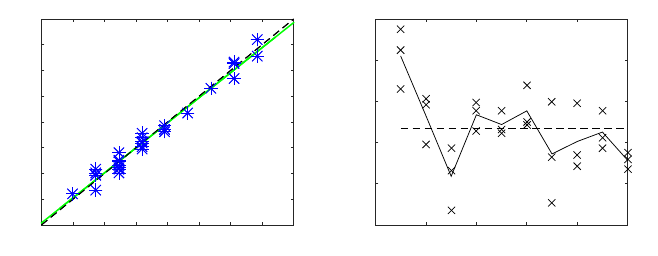
condition. The HR values for both speckle and PPG signal have been plotted in figure
11(a). The linear fitting is almost collinear with the 45 degree line, which demonstrates
the very good agreement between both methods. Finally, the root mean square error
between PPG HR and speckle HR, for all data-sets, was 1.3 bpm.
The results from similarity index are presented in figure 11(b). It is important to
emphasize that PPG and speckle data come from two different sites and two different
information sources. However, they both express the effect of blood flowing through
40
EPS Porto 2017 2017 - European Project Space on Networks, Systems and Technologies
40

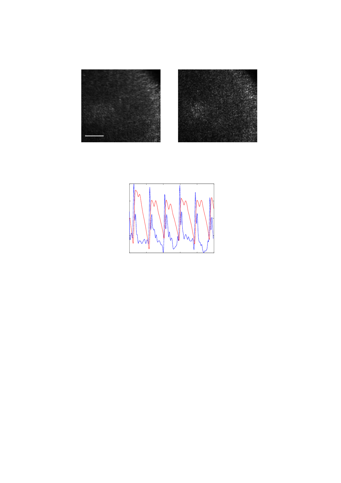
0.5mm
(a) Systole (b) Diastole
Fig. 9. Laser speckle images from the radial artery at different stages of the cardiac cycle: a)
systole, higher skin velocities leading to a blurred speckle image; b) diastole, lower velocities
result in a sharper speckle image.
Time (s)
0 1 2 3 4 5
Amplitude (A.U.)
-1
-0.5
0
0.5
1
Speckle Contrast and PPG signals
Fig. 10. Temporal representation of PPG data (red line) and speckle contrast data (blue line).
the arterial system. For that reason, it is expected to see spectral similarities between
both signals within the range of interest (0-10 Hz). The subject number 1 presents a
very good spectral similarity with all its SI above 0.73. On the contrary, subject num-
ber 3 and 7 present a SI below 0.5. These values show that the precision of the pulse
waveform extraction depends on the analyzed subject. This can be possibly explained
due to the physiological differences between each volunteer, like the blood pressure
and fatty layer. Subjects with lower pressure or large fatty layer lead to a less pulsatile
artery, resulting in lower speckle SNR.
5.3 2D Image Segmentation
The last experiment of this work corresponds to the ones of the 2D image segmentation
study. First, the 4 processing window sizes have been applied to all the data in order
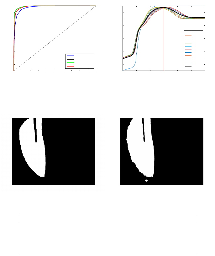
to determine which size performs better. The results have been plotted in figure 12(a).
From this graphic we can conclude that all the methods show very good results with
41
Methods for Hemodynamic Parameters Measurement using the Laser Speckle Effect in Macrocirculation
41

PPG HR (bpm)
50 55 60 65 70 75 80 85 90
Speckle HR (bpm)
50
55
60
65
70
75
80
85
90
speckleHR = 0.97# ppgHR + 1.77
r
2
= 0.97
speckleHR = 0.97# ppgHR + 1.77
r
2
= 0.97
Scatter plot
(a)
Subject
0 2 4 6 8 10
Normalized SI
0.4
0.5
0.6
0.7
0.8
0.9
SI distribution
(b)
Fig. 11. Data analysis: a) HR scatter plot of the PPG HR vs speckle HR. Each star represents one
data set. The black line correspond to the fitting equation and the green line to the first quadrant
bisector. b) Scatter plot of the similarity index (SI) for each subject. The dashed line represents
the total mean and the solid line the subjects mean.
AUC of 0.97, 0.99, 0.99 and 0.98 for window sizes of 3×3, 9×9, 27×27, and 81×81
respectively. However, the intermediate sizes have achieved a performance slightly bet-
ter and, since the smaller window sizes are fast to compute, the method with the window
size of 9×9 can be considered the better one.
After the selection of the best method, the training data-set has been used to select
the best threshold. In oder to achieve this, all the possible thresholds (0-6) were applied
to all the data-set images. The results for each threshold and image was compared with a
manually segmented mask in oder to compute the accuracy of the method. This data is
represented in figure 12(b) where each line represents the evolution of the accuracy
for each data-set image. The best threshold has been determined by computing the
maximum mean accuracy for all the data-set (bold line of figure 12(b)) and corresponds
to 2.95.
Figure 13 shows two segmented images of the moving membrane, one manually
(figure 13(a)) and the other using the automatic entropy based method (figure 13(b)).
The equivalence between both segmentations is evident and, in fact, the entropy based
method could segment even a larger area of the membrane. The black vertical line
corresponds to a dark zone where speckle pattern is not visible (please consult [30] for
more details).
The results of the applications of this method to the validation data-set are presented
in table 3. From this results, it can be concluded that all the evaluation metrics achieved
very good values. In this type of data, there are much more stopped pixels than moving
pixels (class unbalancing) and, in these cases, the MCC must be used to assess the met-
hod quality. This metric ranges from -1 to 1, meaning complete agreement (1), complete
disagreement (-1), and random classifier (0). In this validation data-set, the MCC range
from 0.84 to 0.95 which indicates a very good classifier. Regarding the accuracy, it can
be highlighted that at leas 95% of all the image pixels have been correctly classified.
42
EPS Porto 2017 2017 - European Project Space on Networks, Systems and Technologies
42

0 0.1 0.2 0.3 0.4 0.5 0.6 0.7 0.8 0.9 1
(1-SP)
0
0.1
0.2
0.3
0.4
0.5
0.6
0.7
0.8
0.9
1
SE
ROC curves
3#3 window
9#9 window
27#27 window
81#81 window
(a)
0 1 2 3 4 5 6
Threshold
0
10
20
30
40
50
60
70
80
90
100
Accuracy (%)
Best threshold identi-cation
07m/s
597m/s
987m/s
1177m/s
1477m/s
1957m/s
2357m/s
2937m/s
3527m/s
5867m/s
8807m/s
17597m/s
MeanAC
(b)
Fig. 12. Model optimization: (a) Best element size identification using ROC curves. SE stands for
sensibility and SP for specificity. (b) Best threshold identification for the 9×9 method using 12
images of the training data-set. The vertical red line represents the best threshold (2.95).
Fig. 13. Output of the application a 2.95 threshold.
Table 3. Results in the validation data set-for a window of 9 × 9 pixels.
Movement Max. Vel. (mm/s) AC (%) PPV(%) NPV(%) MCC No. frames
1/5 Hz - 1V
pp
0.06 96.54 86.26 99.03 0.8872 30
1 Hz - 1V
pp
0.29 98.73 96.16 99.21 0.9519 15
1/3 Hz - 4V
pp
0.59 97.57 94.95 98.13 0.9178 45
1/2 Hz - 6V
pp
0.88 95.80 92.96 96.33 0.8512 30
1 Hz - 4V
pp
1.17 95.14 78.04 99.34 0.8416 15
6 Conclusion
This chapter presented three different studies that demonstrate the capacity of LSI to
assess macrocirculatory information. These experiments were initiated by using a bench
phantom that mimics the arterial vibrations and ended in real in vivo applications using
the same methods used in commercially available LSI devices.
All the results demonstrated that LSI can be used with good reliability to extract
macrocirculation parameters. The main purposes of this project was to proof that the
available LSI devices that are used for microcirculation assessment could also be used
for macrocirculation assessment without making big hardware and software changes.
43
Methods for Hemodynamic Parameters Measurement using the Laser Speckle Effect in Macrocirculation
43

With the inclusion of this feature in LSI devices, a new macro-micro circulatory joint
information could be assessed and explored.
References
1. Ozcan, A., Bilenca, A., Desjardins, A.E., Bouma, B.E., Tearney, G.J.: Speckle reduction in
optical coherence tomography images using digital filtering. Journal of the Optical Society
of America. A, Optics, image science, and vision 24 (2007) 1901–1910
2. Gr
´
ediac, M.: The use of full-field measurement methods in composite material characteri-
zation: interest and limitations. Composites Part A: Applied Science and Manufacturing 35
(2004) 751–761
3. Bendjus, B., Cikalova, U., Schreiber, J.: Material characterization by laser speckle photome-
try. In: V International Conference on Speckle Metrology. Volume 8413., Vigo, Spain, SPIE
(2012) 841315
4. Fercher, A., Briers, J.: Flow visualization by means of single-exposure speckle photography.
Optics Communications 37 (1981) 326–330
5. Boas, D.a., Dunn, A.K.: Laser speckle contrast imaging in biomedical optics. Journal of
biomedical optics 15 (2010) 011109
6. Parthasarathy, A.B., Tom, W.J., Gopal, A., Zhang, X., Dunn, A.K.: Robust flow measurement
with multi-exposure speckle imaging. Optics express 16 (2008) 1975–89
7. Kazmi, S.M.S., Wu, R.K., Dunn, A.K.: Evaluating multi-exposure speckle imaging estimates
of absolute autocorrelation times. Optics letters 40 (2015) 3643–3646
8. Ramirez-San-Juan, J., Regan, C., Coyotl-Ocelotl, B., Choi, B.: Spatial versus temporal laser
speckle contrast analyses in the presence of static optical scatterers. Journal of Biomedical
Optics 19 (2014) 106009–106009
9. Zakharov, P., V
¨
olker, A.C., Wyss, M.T., Haiss, F., Calcinaghi, N., Zunzunegui, C., Buck, A.,
Scheffold, F., Weber, B.: Dynamic laser speckle imaging of cerebral blood flow. Optics
express 17 (2009) 13904–13917
10. Varma, H.M., Valdes, C.P., Kristoffersen, A.K., Culver, J.P., Durduran, T.: Speckle contrast
optical tomography: A new method for deep tissue three-dimensional tomography of blood
flow. Biomedical Optics Express 5 (2014) 1275–1289
11. Huang, C., Irwin, D., Lin, Y., Shang, Y., He, L., Kong, W., Luo, J., Yu, G., Huang, C., Irwin,
D., Lin, Y., Shang, Y., He, L., Kong, W.: Speckle contrast diffuse correlation tomography of
complex turbid medium flow. Medical physics 42 (2015) 4000–4006
12. Senarathna, J., Member, S., Rege, A., Li, N., Thakor, N.V.: Laser Speckle Contrast Imaging
: Theory , Instrumentation and Applications. Biomedical Engineering, IEEE Reviews in 6
(2013) 99–110
13. Briers, D., Duncan, D., Kirkpatrick, S., Larsson, M., Stromberg, T., Thompson, O.: Laser
speckle contrast imaging : theoretical and practical limitations. Journal of Bomedical Optics
18 (2013) 1–9
14. Vaz, P.G., Humeau-Heurtier, A., Figueiras, E., Correia, C., Cardoso, J.: Laser speckle ima-
ging to monitor microvascular blood flow: a Review. IEEE Reviews in Biomedical Engi-
neering In press (2016) 1–1
15. Liu, J., Zhang, H., Lu, J., Ni, X., Shen, Z.: Quantitative model of diffuse speckle contrast
analysis for flow measurement. Journal of Biomedical Optics 22 (2017) 76016
16. Ponticorvo, A., Burmeister, D.M., Rowland, R., Baldado, M., Kennedy, G.T., Saager, R.,
Bernal, N., Choi, B., Durkin, A.J.: Quantitative long-term measurements of burns in a rat
model using Spatial Frequency Domain Imaging (SFDI) and Laser Speckle Imaging (LSI).
Lasers in Surgery and Medicine 49 (2017) 293–304
44
EPS Porto 2017 2017 - European Project Space on Networks, Systems and Technologies
44

17. Liu, Q., Chen, S., Soetikno, B., Liu, W., Tong, S., Zhang, H.: Monitoring acute stroke in
mouse model using laser speckle imaging-guided visible-light optical coherence tomography
(2017)
18. Zakharov, P.: Ergodic and non-ergodic regimes in temporal laser speckle imaging. Optics
Letters 42 (2017) 2299–2301
19. Kirkpatrick, S., Duncan, D., Wang, R., Hinds, M.: Quantitative temporal speckle contrast
imaging for tissue mechanics. Journal of the Optical Society of America. A, Optics, image
science, and vision 24 (2007) 3728–3734
20. Duncan, D.D., Kirkpatrick, S.J.: Can laser speckle flowmetry be made a quantitative tool?
Journal of the Optical Society of America. A, Optics, image science, and vision 25 (2008)
2088–2094
21. Briers, J.D., Fercher, A.F.: Retinal blood-flow visualization by means of laser speckle pho-
tography. Investigative ophthalmology & visual science 22 (1982) 255–259
22. Thompson, O., Andrews, M., Hirst, E.: Correction for spatial averaging in laser speckle
contrast analysis. Biomedical Optics Express 2 (2011) 1021–1029
23. Ennos, A.E.: Speckle interferometry. In: Laser Speckle and Related Phenomena. Volume 9
of Topics in Applied Physics. Springer Berlin Heidelberg (1975) 203–253
24. Khaksari, K., Kirkpatrick, S.J.: Combined effects of scattering and absorption on laser
speckle contrast imaging. Journal of Biomedical Optics 21 (2016) 76002
25. Williams, B., Lacy, P.S., Thom, S.M., Cruickshank, K., Stanton, A., Collier, D., Hughes,
A.D., Thurston, H., O’Rourke, M.: Differential impact of blood pressure-lowering drugs
on central aortic pressure and clinical outcomes: Principal results of the Conduit Artery
Function Evaluation (CAFE) study. Circulation 113 (2006) 1213–1225
26. Pereira, T., Santos, I., Oliveira, T., Vaz, P., Correia, T., Pereira, T., Santos, H., Pereira, H., Al-
meida, V., Cardoso, J.: Characterization of optical system for hemodynamic multi-parameter
assessment. Cardiovascular Engineering and Technology 4 (2013) 87–97
27. Vaz, P.: Methods for hemodynamic parameters measurement using the laser speckle effect
in macro and microcirculation. Phd thesis (available online with credentials), Universidade
de Coimbra (2016)
28. Vaz, P., Pereira, T., Figueiras, E., Correia, C., Humeau-Heurtier, A., Cardoso, J.: Which
wavelength is the best for arterial pulse waveform extraction using laser speckle imaging?
Biomedical Signal Processing and Control 25 (2016) 188–195
29. Vaz, P., Santos, P., Figueiras, E., Correia, C., Humeau-Heurtier, A., Cardoso, J.: Laser
speckle contrast analysis for pulse waveform extraction. In: Novel Biophotonics Techni-
ques and Applications III. Volume 9540., Munich, SPIE (2015) 954006–954007
30. Vaz, P., Pereira, T., Capela, D., Requicha, L., Correia, C., Humeau-Heuertier, A., Cardoso,
J.: Use of laser speckle and entropy computation to segment images of diffuse objects with
longitudinal motion. In: II International Conference on Applied Optics and Photonics, Aveiro
(2014)
45
Methods for Hemodynamic Parameters Measurement using the Laser Speckle Effect in Macrocirculation
45