A Real-Time Edge-Preserving Denoising Filter
Simon Reich
1
, Florentin W
¨
org
¨
otter
1
and Babette Dellen
2
1
Third Institute of Physics - Biophysics, Georg-August-Universit
¨
at G
¨
ottingen,
Friedrich-Hund-Platz 1, 37077 G
¨
ottingen, Germany
2
Hochschule Koblenz, Joseph-Rovan-Allee 2, 53424 Remagen
Keywords:
Edge-Preserving, Denoising, Real-Time.
Abstract:
Even in todays world, where augmented reality glasses and 3d sensors become rapidly less expensive and
widely more used, the most important sensor remains the 2d RGB camera. Every camera is an optical device
and prone to sensor noise, especially in dark environments or environments with extreme high dynamic range.
The here introduced filter removes a wide variation of noise, for example Gaussian noise and salt-and-pepper
noise, but preserves edges. Due to the highly parallel structure of the method, the implementation on a GPU
runs in real-time, allowing us to process standard images within tens of milliseconds. The filter is first tested
on 2d image data and based on the Berkeley Image Dataset and Coco Dataset we outperform other standard
methods. Afterwards, we show a generalization to arbitrary dimensions using noisy low level sensor data. As
a result the filter can be used not only for image enhancement, but also for noise reduction on sensors like
acceleremoters, gyroscopes, or GPS-trackers, which are widely used in robotic applications.
1 INTRODUCTION
Real-time computer vision in fast moving robots still
remains a challenging task, especially when forced to
use limited computing power, as it is usually the case
when implemented on embedded systems. Different
light conditions are just one aspect of this vast field of
problems. Cameras (analog as well as digital cameras)
introduce noise in poor light conditions, meaning in
environments with low signal-to-noise ratio.
Removing this noise usually leads to better perfor-
mance of object recognition tasks in 2d and 3d ima-
ges, more stable computation of features, and improve
tracking results. It was shown (Reich et al., 2013)
that removal of texture from 2d images significantly
improves image segmentation results.
An additional application is the automatic pro-
duction of images, which are, generally speaking,
more appealing to humans; there is a big community of
photographers and we deem removing noise for pure
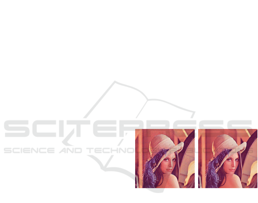
aesthetic value as also important. One application of
the here presented filter is shown in Fig. 1.
Still, the filter generalizes well on arbitrary dimen-
sions. In a second part we will show how to apply
the same mechanisms to an arbitrary number of di-
mensions, enabling the filter to run on any physical
measurement, for example on 1d sensor data obtained
(a) Noisy test image. (b) Denoised test image.
Figure 1: Even today, denoising remains a challenging task.
Here, we propose a novel, real-time denoising filter, which
we call Edge-Preserfing-Filter (EPF).
from an accelerometer, gyroscope, or GPS tracker.
Removing noise is a two-step process: First a noisy
pixel needs to be detected, second it needs to be smoot-
hed out. Both steps offer a wide range of problems.
In the first step we need to define a noisy pixel in a
mathematical sense, such that a computer can under-
stand what we are looking for. This means that we
will need to define a similarity criterion. However,
similarities can exist on different scales, i.e. between
adjacent pixels or groups of pixels, as it is the case
for texture. In the second step a target value needs
to be computed, which replaces the noisy pixel. This
target value should, again, only depend on the local
Reich, S., Wörgötter, F. and Dellen, B.
A Real-Time Edge-Preserving Denoising Filter.
DOI: 10.5220/0006509000850094
In Proceedings of the 13th International Joint Conference on Computer Vision, Imaging and Computer Graphics Theory and Applications (VISIGRAPP 2018) - Volume 4: VISAPP, pages
85-94
ISBN: 978-989-758-290-5
Copyright © 2018 by SCITEPRESS – Science and Technology Publications, Lda. All rights reserved
85

neighborhood.
Removing noise has a long history in science. Most
notable is the Gaussian Filter. It works by convolving
an image with a Gaussian function and thus works as
a simple low-pass filter, attenuating high frequency
signals (Gonzalez and Woods, 2002, p. 257f). As
edges are also a high-frequency signal, they will be
blurred out, too.
Noise in images is usually distinguished using a
threshold. This thresholds can be either learned using
a training set of images, as in support vector machines
(Yang et al., 2010) and neural networks (Muneyasu
et al., 1995; Pandey et al., 2016), or the threshold may
be computed from the surrounding pixel values, as in
(Du et al., 2011). (Lev et al., 1977) identified similar
pixels by detecting edges and itertively replacing the
intensity of the pixel by the mean of all pixels in a
small environment.
Another approach is presented in (Tomasi and Man-
duchi, 1998): The so called bilateral filter blurs neig-
hboring pixels depending on their combined color and
spatial distance. Hence, texture and noise, which has
small deviation from the mean can be blurred without
affecting boundaries. This leads to a trade-off: large
blurring factors are needed to smooth out high level
of noise, having the consequence that edges are not
preserved anymore.
Another wide class of algorithms denoise by aver-
aging. This averaging may happen locally as in the
Gaussian smoothing model (Lindenbaum et al., 1994),
the anisotropic smoothing model (Perona and Malik,
1990; Alvarez et al., 1992), based on neighborhood
filtering as in the already mentioned bilateral filter
(Tomasi and Manduchi, 1998), using local variations
as in (Rudin et al., 1992), or based on the wavelet
thresholding method (Donoho, 1995).
All this powerful methods have one common draw-
back: they all smooth small scaled noise and preserve
color edges, although however are not able to distin-
guish between a color edge and large scaled noise, e.g.
outliers. Outliers are a common problem in any sensor
based application, as in accelerometers or gyroscopes,
but also in 2d-rgb cameras, where high ISO settings
often pose a big problem. More recent methods, which
achieve this goal (Dabov et al., 2007; Zoran and Weiss,
2011; Mairal et al., 2009), do not perform in real-time.
The here presented approach has the following featu-
res: (1) smooths out small scaled noise, (2) smooths
out outliers, (3) still preserves color edges, and (4)
performs in real-time.
In the following section, we introduce a mathe-
matical formulation of our filter in the discrete and
continuous domain. Afterwards, we will utilize the
algorithm using artificial noise on an image data sets
and compare the results. Then, we describe the genera-
lization on benchmark data and perform experiments
on artificial data. This will be followed by a detailed
discussion and conclusion.
2 METHOD
Let Φ(i) be our observed image. Then our noisy image
is defined as
Φ(i) = u(i) + n(i), (1)
where u(i) is the “true” value and n(i) is the noise at
image position i . Here, we will model noise as Gaus-
sian white noise, meaning n(i) is Gaussian distributed
with zero mean and variance σ
2
. Additionally we will
add salt-and-pepper noise: a fixed percentage of color
channels will be set to either 0 or its maximum va-
lue. We define our filter D
h
, with filter parameter h , as
follows
Φ = D
h
(Φ) + n (2)
meaning, that for an optimal filter
u = D
h
(u + n) (3)
should be true. The filter parameter h should depend
only on the variance of the noise h = h(σ) . Later, for
evaluation the Root-Mean-Square Error (RMSE) and
Peak Signal-to-Noise Ratio (PSNR) between u and
D
h
(u + n) is computed.
2.1 Proposed Filter
A flowchart of the proposed filter is shown in Fig. 2.
First, the image Φ is divided into subwindows Ψ si-
zed N = k · l , where each subwindow is shifted by one
pixel relative to the last one, such that there are as
many subwindows as there are pixels in the image.
Each subwindow is then smoothed using a Gaussian
kernel. Subwindow size k ×l and Gaussian smoothing
parameter are hyperparameters, which need to be ma-
nually set. However, all three heavily depend on the
amount of noise you would want to remove. For each
subwindow centered around pixel position (i, j) a dis-
tance matrix ∆
i, j
and a mean distance δ
m
i, j
is computed
in the color domain. This offers a measurement for
noise, as described below. A user selected threshold
τ , which defines a threshold between noise and a mere
color edge, is applied to ∆
i, j
and δ
m
i, j
. In case of noise,
a weight ω
i, j
is computed, which will move the color
values of the pixel in the subwindow to the mean color
of the subwindow.
VISAPP 2018 - International Conference on Computer Vision Theory and Applications
86

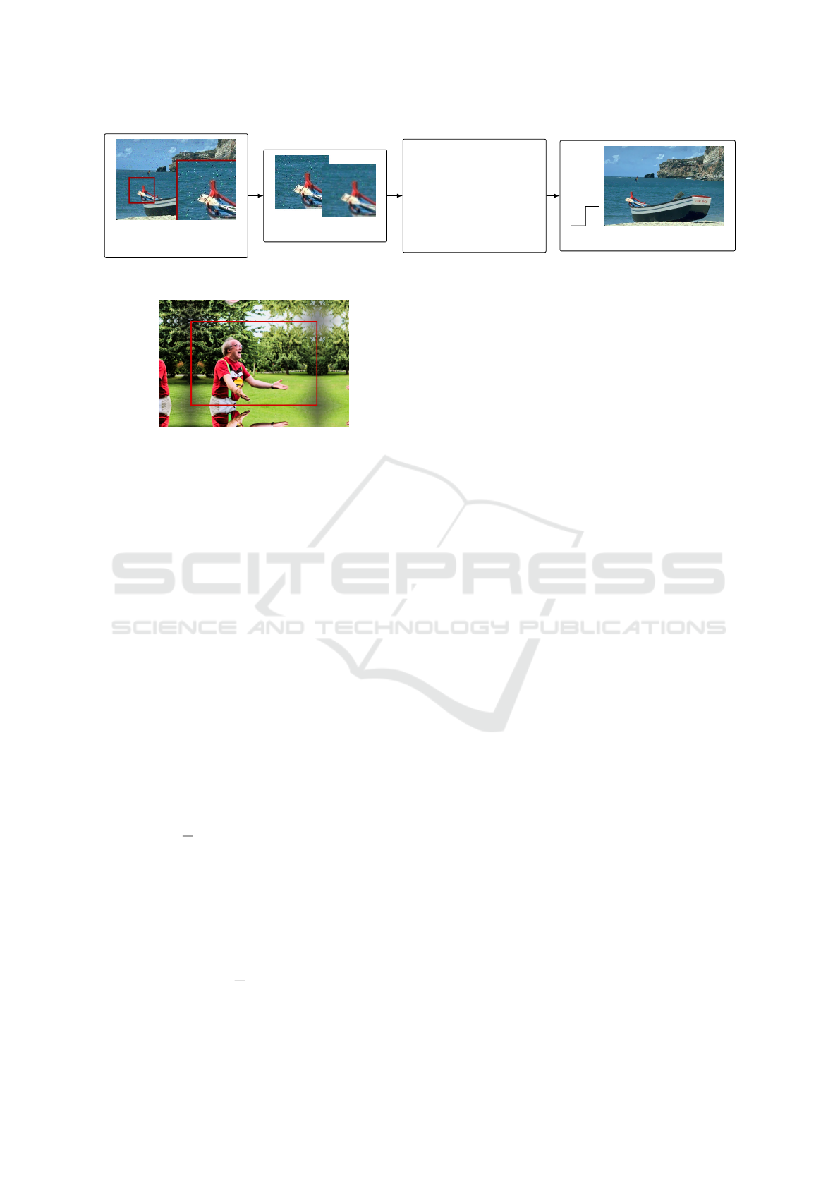
a) Division into
subwindows Ψ
b) Smoothing



δ
0,0
δ
0,1
... δ
0,k
δ
1,0
δ
1,1
...
... ...
δ
l,0
... δ
l,k



c) Compute distance
matrix ∆ and δ
m
d) Apply threshold τ
Figure 2: Overview of the system structure. A detailed explanation of all steps is shown in section 2.
Figure 3: Peridiodic mirrored boundary conditions are used
for image subwindows. Red rectangle denotes borders of
original image.
Division into Subwindows. Let one pixel at po-
sition (i, j) contain the color information ϕ
ϕ
ϕ
i, j
=
(ϕ
r
i, j
ϕ
g
i, j
ϕ
b
i, j
)
T
. We create a subwindow Ψ
(i, j)
around
(i, j) , such that (i, j) is centered. In case we hit an
image boundary, periodic mirrored boundary conditi-
ons are used as visualized in Fig. 3. The size of the
subwindow is defined by k × l and pixel position in-
side the subwindow will be denoted by (r,s) , such that
0 ≤ r < k and 0 ≤ s < l.
Smoothing. Each subwindow is smoothed via a
Gaussian kernel (Gonzalez and Woods, 2002, p. 257f).
This removes outliers, which would otherwise distort
the computation of the mean as described in the next
step.
Computation of the Distance Matrix. For each
subwindow Ψ
(i, j)
the arithmetic mean is calculated
as
ψ
ψ
ψ
(i, j)
m
=
1
N
∑
r,s
ψ
r
r,s
∑
r,s
ψ
g
r,s
∑
r,s
ψ
b
r,s
!
T
(4)
where N = k · l denotes the size of the subwindow. The
pixelwise distances
δ
(i, j)
r,s
= |ψ
ψ
ψ
r,s
− ψ
ψ
ψ
(i, j)
m
|
2
(5)
are stored in a matrix ∆
(i, j)
. Furthermore, for each
subwindow Ψ
(i, j)
the mean pixelwise distance
δ
(i, j)
m
=
1
N
∑
r,s
δ
(i, j)
r,s
(6)
is calculated.
Thresholding. Using a threshold we will now ana-
lyze, whether a subwindow contains a color edge (and
therefore no pixels should be smoothed), one pixel con-
tains an outlier (and should be corrected), or neither,
which means the pixel value should also not be repla-
ced. If δ
(i, j)
m
is large, we have a subwindow with big
color variations. This means we have found a subwin-
dow, which holds a color edge. If δ
(i, j)
m
is small, but
one single pixel holds a big color variations (large
δ
(i, j)
r,s
), we have found an outlier, which needs to be
replaced. If both, δ
(i, j)
m
and δ
(i, j)
r,s
are small, the pixel
holds a “normal color” value. We can now introduce
a threshold τ to identify noisy pixels and color edges,
yielding
ψ
r,s
=





color edge , if δ
(i,j)
m
> τ,
noise , if δ
(i,j)
m
≤ τ and δ
r,s
> τ,
neither , else.
(7)
Update of RGB Values.
A new image Θ , holding
the pixel values θ
θ
θ
i, j
is computed based upon the squa-
red distance of the user based threshold τ and the pixe-
lwise distance δ
r,s
. θ
θ
θ
i, j
is updated as follows
θ
θ
θ
i, j
←− θ
θ
θ
i, j
+ ψ
r,s
·

τ − δ
(i, j)
r,s

2
· ψ
ψ
ψ
(i, j)
m
. (8)
Please note, that due to the sliding subwindows each
pixel is updated N = k · l times and therefore needs
to be normalized. Thus, an additional weight Ω is
introduced for each pixel ω
i, j
as
ω
i, j
←− ω
i, j
+ ψ
r,s
·

τ − δ
(i, j)
r,s

2
. (9)
The final image results from division of Θ by Ω . In
rare cases τ = δ
(i, j)
r,s
for large image patches can happen,
which will result in ω
i, j
= 0 according to (9) . To avoid
division by zero we suggest to initialize Ω with ones
instead of zeros (since in general ω
i, j
 0 , this does
not change the final outcome significantly).
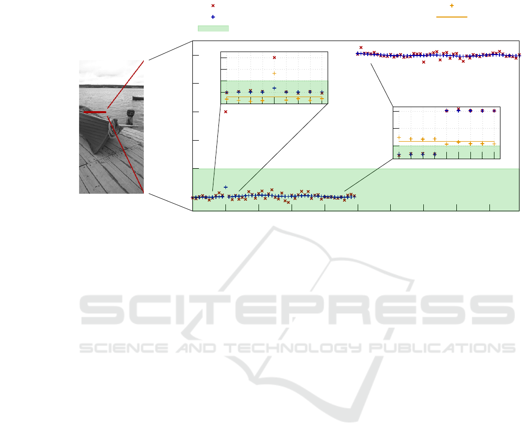
An example for these subwindows can be seen
in Fig. 4. For demonstration purposes a simple 1d
grayscale image holding 100 pixels is shown. Each
pixel has low variance Gaussian noise added. Pixel 10
A Real-Time Edge-Preserving Denoising Filter
87

10
20
30
40
50
60
0 10 20 30 40 50 60 70 80 90
grayscale value
pixel number
0
10
20
30
40
Original Data
Filtered Data
Threshold τ
pixelwise color distance δ
r,s
mean pixelwise color distance δ
m
20
40
60
Figure 4: On the left a grayscale image, which needs to be filtered, is shown. For visualization purposes 100px (marked in red)
are chosen for detailed analysis and plotted in the large graph. Each pixel has Gaussian noise (variance of 1) added, additionally
pixel 10 contains an outlier. At pixel 50 there is a color edge. In blue the same pixels are shown after being processed by
the filter. The left subplot contains one subwindow sized 9 × 1px . Pixel 10 is smoothed out, since the mean pixelwise color
distance δ
m
is low and thus pixel 10 is identified as noise. The right subgraph shows another subwindow, which detects of a
color edge. δ
m
is greater than threshold τ and therefore no values are smoothed inside this subwindow.
was manually set to a significant higher value; at pixel
50 a color edge begins. Noisy pixel 10 is identified,
since the mean pixelwise color distance δ
m
is quiet low,
while the pixelwise color distance δ
r,s
is large; thus
pixel 10 is smoothed out. At the color edge the mean
pixelwise distance is greater than the threshold δ
m
> τ ,
which is interpreted correctly as a color edge and thus
no value in the shown subwindow is smoothed out.
However, one problem arises, when the subwindow
contains only one pixel from the color edge. This one
pixel cannot safely be differentiated between noise
and color edge – even for a human this would be an
impossible task. Therefore, pixels at the border of the
subwindow are not smoothed, when detected as noise.
2.2 Formulation of the Proposed Filter
in the Continuous Domain
Let f
f
f (x
x
x) define the smoothed input image, h
h
h(x
x
x) the
output image, c
c
c(ζ
ζ
ζ, x
x
x) measures the geometric close-
ness and s
s
s( f
f
f (ζ
ζ
ζ), f
f
f (x
x
x)) the photometric similarity. As
we want to address specifically color images, bold
letters refer to RGB-vectors. In this section | · | also
refers to per-element-multiplication instead of vector
multiplication. In our approach we first want to detect
noise based on a user defined parameter τ . If noise is
detected, we want to remove it, and in case of a color
edge, we want to preserve the edge. Therefore, we
define a mean value
m
m
m(x
x
x) = k
k
k
−1
m
(x
x
x)
Z
∞
−∞
Z
∞
−∞
f
f
f (ζ
ζ
ζ) · c
c
c(ζ
ζ
ζ, x
x
x)dζ
ζ
ζ
k
k
k
m
(x
x
x) =
Z
∞
−∞
Z
∞
−∞
c
c
c(ζ
ζ
ζ, x
x
x)dζ
ζ
ζ (10)
and a distance function
d ( f
f
f (x
x
x), m
m
m(x
x
x)) =
|
f
f
f (x
x
x) − m
m
m(x
x
x)
|
, (11)
which results in the pixelwise distance. The mean va-
lue m
m
m(x
x
x) now holds the average color value inside a
spatial neighborhood of x
x
x and d holds the color dis-
tance from the pixel to the average m
m
m(x
x
x) . If the spatial
neighborhood holds only small scaled noise we expect
a low pixelwise distance d , as well as a low average
pixelwise distance in the spatial neighborhood c
c
c:
p(x
x
x) = k
−1
p
ZZ
∞
−∞
d ( f
f
f (ζ
ζ
ζ), m
m
m(x
x
x))c
c
c(ζ
ζ
ζ, x
x
x)dζ
ζ
ζ
k
p
(x
x
x) =
ZZ
∞
−∞
c
c
c(ζ
ζ
ζ, x
x
x)dζ
ζ
ζ. (12)
Therefore, we can make a decision using a thres-
VISAPP 2018 - International Conference on Computer Vision Theory and Applications
88

hold τ as
h
h
h(x
x
x) = k
k
k
−1
R
(x
x
x) ·





RR
∞
−∞
f
f
f (ζ
ζ
ζ) · c
c
c(ζ
ζ
ζ, x
x
x) · s
s
s(ζ
ζ
ζ, x
x
x)dζ
ζ
ζ p ≤ τ
RR
∞
−∞
f
f
f (ζ
ζ
ζ) · c
c
c(ζ
ζ
ζ, x
x
x) · s
s
s(ζ
ζ
ζ, x
x
x)dζ
ζ
ζ p ≤ τ,d > τ
RR
∞
−∞
f
f
f (ζ
ζ
ζ) · c
c
c(ζ
ζ
ζ, x
x
x)dζ
ζ
ζ else,
where k
R
is the respective normalization. d can now
be used to distinguish large scale noise. We used a 2d
step function
c
c
c(ζ
ζ
ζ, x
x
x) =
(
1 x
x
x − a
a
a ≤ ζ
ζ
ζ ≤ x
x
x + b
b
b
0 else
, (13)
using the conditions a
a
a,b
b
b,e
e
e ∈ R
2
≥0
|a
a
a + b
b
b = e
e
e with a
fixed e
e
e . This generates a rectangle of the size e
e
e around
x
x
x . As this definition is not feasable in the continuous
domain as it generates a nonfinite number of subwin-
dows to calculte, in the discrete case however every
pixel is checked and updated according to its neighbor-
hood e
e
e . As a measure for similarity we used a squared
distance
s
s
s((ζ
ζ
ζ), x
x
x) = (τ − d( f
f
f (x
x
x), m
m
m(x
x
x)))
2
|m
m
m(x
x
x)| (14)
and the euclidian norm. In case of noise detection the
output is moved to the mean. The maximum size of
the step can be adjusted via the threshold τ.
2.3 Real-time Implementation
The proposed filter can only run in real-time on parallel
hardware, since the computation of multiple subwin-
dows is very intensive on traditional CPUs. Still, once
the image Φ is read, values for the subwindows Ψ
(i, j)
can be computed independently. For acceleration we
use a graphics processor unit (GPU).
In our approach the images are filtered using a
subwindow of size k, l = 10 . As ∆ and δ
(i, j)
m
are calcu-
lated over each subwindow, this also sets the maximum
size of noise that is detected. We tested two implemen-
tations of the algorithm: The CPU measurement refers
to a single-threaded implementation using an Intel i7-
3930K twelve-core processor at 3,2 GHz using one
core and 16 GB RAM. The GPU version is executed
on an Nvidia GTX580 graphics card using 512 cores
and 1.5 GB device memory.
3 EXPERIMENTS
In this section, we will first look at the user controlled
parameters, the subwindow size N and the threshold τ .
The Gaussian smoothing parameters, which are also
hyperparameters, heavily depend on the data type: is
the filter too strong, the final image will be blurry; a
filter too weak will not smooth enough. We found a
kernel size of 5px and σ = 0.3 working very well for
all images in the datasets. Afterwards, we will com-
pare our proposed filter to the bilateral filter, simple
Gaussian kernel, Median filter, and Non-local-means
filter. Lastly, we will look into the computational com-
plexity and real-time implementations.
3.1 Subwindow Size
First, we will have a look at the effect of the most impo-
rant user controlled parameter: the size of the subwin-
dow N . Since each pixel is N times checked, the com-
putational complexity increases linearly with N . This
parameter also controls the amount of noise, which
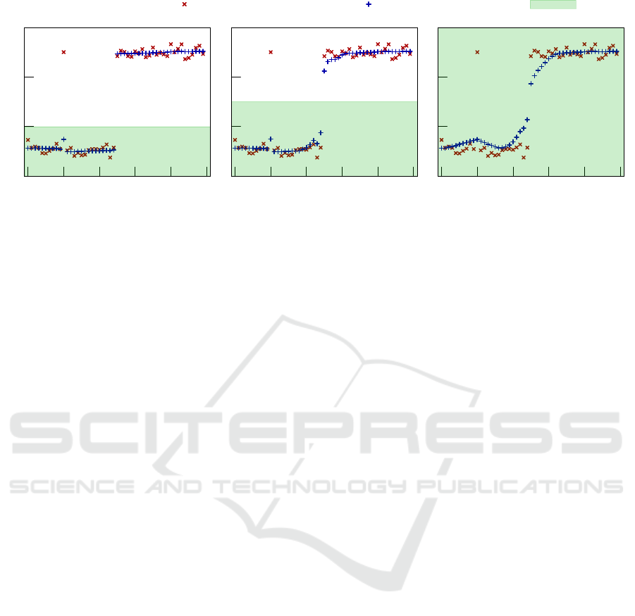
is either classified as noise or color edge. In Fig. 5 a
one dimensional grayscale image is shown and filtered
using three different subwindow sizes N = 3,9, 15 px .
For each size the color edge is preserved. For N = 3px ,
Fig. 5a, the filter follows the data more closely; this
also means that an outlier, as shown in pixel 10 in the
data sample, has a greater influence on the filtered data.
For a subwindow size of N = 9px , see Fig. 5b, the data
is more heavily smoothed and the outlier is almost not
visible in the filtered data. In Fig. 5c a subwindow size
of N = 29 px was chosen. Since the color edge begins
at pixel 26, it will be alwasy present in all subwindows
of all left sided pixels due to the periodic boundary
conditions. Additionally, the outlier on the left side
increases the mean pixelwise distance, such that the
left side is almost not smoothed at all. Only the right
side, which does not contain the artificial outlier, is
smoothed.
Thus, the subwindow controls the spatial size of a
color edge to be detected.
3.2 Threshold τ
τ
τ
Next, we will analyze the effect of the threshold τ ,
this is depicted in Fig. 6. As shown in section 2, τ
controls the maximum step size for detecting noise
and color edges. In Fig. 6a a threshold of τ = 10 is
used, which is small enough to detect the color step.
A larger threshold of τ = 15 , used in Fig. 6b, already
introduces some smoothing at the color edge. Please
also note, that the outlier pixel at position 10 is not
any more detected as noise; instead it has significant
effect on the smoothing of its neighboring pixels. A
large threshold of τ = 30 can be seen in Fig. 6c; 30
is by far bigger than any data point and consequently
everything will be smoothed. The color edge is not
preserved any more.
A Real-Time Edge-Preserving Denoising Filter
89

Original Data Filtered Data Threshold τ
0
10
20
0 10 20 30 40 50
(a) Subwindow size of N = 3px.
0
10
20
0 10 20 30 40 50
(b) Subwindow size of N = 9px.
0
10
20
0 10 20 30 40 50
(c) Subwindow size of N = 29px.
Figure 5: Shown is the effect of different subwindow sizes on one data set: a one dimensional grayscale image containing a
color edge at pixel 25 and one outlier at pixel 10. In Fig. 5a a subwindow size of 3 px is shown. The data is smoothed and the
color edge is preserved. The oulier at pixel 10, however, is also smoothed, but has also some effect on the neighboring pixels.
A subwindow size of 9 px, as shown in Fig. 5b, seems to be more fitting: the outlier is smoothed and the color edge preserved.
Fig. 5c shows a subwindow size of 29 px. The data on the left side is not smoothed, since the color edge and the outlier are
always in one subwindow and thus the mean pixelwise color distance is greater than the threshold τ . This means the left side is
always detected as “containing a color edge”. The right side of the data is smoothed, due to the periodic boundary conditions.
Thus, the threshold τ controls the maximum height
of a color edge to be detected.
3.3 Application to 2D images
We corrupted our images by first adding Gaussian
distributed noise to each pixel and each color channel
using a standard deviation of σ
c
= 5 . Additionally, we
added salt-and-pepper noise (s&p noise) to one color
channel of 4% of all pixels. We tested on the Berkeley
Segmentation Dataset and Benchmark (Arbelaez et al.,
2011) (500 images) and the 2014 testing set of the
Common Objects in Context Dataset (Coco Dataset)
(Lin et al., 2014) (40775 images).
The corrupted image is then given to a simple Gaus-
sian blurring filter (kernel size: 5 × 5 px, σ
x,y
= 2 ), a
bilateral filter ( σ
c
= 110 , σ
s
= 5 ) (Tomasi and Mandu-
chi, 1998), a median blurring filter (kernel size: 3 px)
(Sonka et al., 2014, p. 129f), a non-local-means filter
( h
d
= 7 px , h
c
= 7 px , template window: 7 × 7 px , se-
arch window: 21 × 21px ) (Buades et al., 2005), and
our proposed filter (subwindow: image size divided
by 150, but at least 10 × 10px , threshold τ = 10 ). The
denoised image is compared to the uncorrupted image
using root-mean-square error (RMSE), defined as
RMSE =
s
∑
n
i=1

φ
original
− φ
denoised

2
n
, (15)
and peak signal-to-noise ratio (PSNR):
PSNR = 20 · log
10

max(φ
original
)
RMSE

. (16)
Table 1: Comparison of RMSE and PSNR computed on the
Berkeley Dataset (500 images) and the Coco Dataset (40775
images). The first line “Original” refers to the not denoised
image. The last digits are uncertain due to rounding errors.
Berkeley Dataset Coco Dataset
RMSE PSNR RMSE PSNR
Original 17.9(5) 23.3(1) 17.3(1) 23.3(3)
EPF 7
7
7.
.
.0
0
0(
(
(6
6
6)
)
) 3
3
31
1
1.
.
.0
0
0(
(
(5
5
5)
)
) 7
7
7.
.
.8
8
8(
(
(9
9
9)
)
) 3
3
30
0
0.
.
.4
4
4(
(
(7
7
7)
)
)
Bilateral 10.4(1) 27.7(5) 10.4(3) 28.0(1)
Gaussian 14.5(9) 25.0(8) 15.6(9) 24.8(1)
Median 14.0(4) 25.6(3) 14.9(1) 25.5(4)
NLM 11.4(0) 26.8(6) 12.2(8) 26.4(4)
All filter parameters listed above were chosen to mini-
mize RMSE and maximize PSNR. Results are shown
in Tab. 1 and will be discussed in the next section.
Image examples are provided in figure 7.
The proposed filter achieves on both datasets the
best performance markers. In the discussion, section 4,
we will compare our results to more recent, state-of-the
art algorithms.
3.4 Application to 1D Sensor Data
As already suggested in Fig. 4, 5, and 6, the filter can
also be applied to 1D data. This may happen, for exam-
ple, as a post-processing step for sensor readings. We
have tested the filter on three different settings: first,
an alternating line, which switches every 100 samples
its height to either f (x) = f
min
or f (x) = f
max
; second,
a sawtooth wave defined by f (x) = x − floor
100
(x) l;
and third, a sinusoidal wave f (x) = sin2πx/250 with
a wave length of 250 data points. Every data line
VISAPP 2018 - International Conference on Computer Vision Theory and Applications
90

Original Data Filtered Data Threshold τ
0
10
20
0 10 20 30 40 50
(a) Threshold of τ = 10.
0
10
20
0 10 20 30 40 50
(b) Threshold of τ = 15.
0
10
20
0 10 20 30 40 50
(c) Threshold of τ = 30.
Figure 6: Shown is the effect of three different thresholds on one data set: a one dimensional grayscale image containing a
color edge at pixel 25 and one outlier at pixel 10. The subwindow size is N = 9 px . In Fig. 6a a threshold of τ = 10 is used.
The outlier is detected as such and smoothed and the color edge is preserved. In Fig. 6b, however, the outlier at pixel 10 is not
detected as such; it raises the average pixel value of the subwindows and has great influence on the smoothing: all pixels in
its local neighborhood have an increased value after smoothing. Also the color edge is not preserved any more. This effect
becomes even more visible in Fig. 6c, where heavy smoothing is applied to the color edge.
consists of a total length of 1000 samples. To each
scenario either Gaussian noise with variance of σ = 10 ,
salt-and-pepper noise (to 5% of samples), or both is
added.
Again, we compared our proposed filter ( N = 11 ,
τ = 30 ) to a Gaussian blurring filter (kernel: 7 × 7 px,
σ
x,y
= 3 ), a bilateral filter ( σ
c
= 30 , σ
s
= 30 , and a
median filter (kernel size: 9 px). We computed RMSE
and PSNR according to (15) and (16) . Results are
shown in Tab. 2.
In almost all experiments we outperform other stan-
dard 1d filtering methods. While the median filter per-
forms very well on salt-and-pepper noise, it is not edge
preserving and thus introduces artefacts on edges. The
bilateral filter on the other hand, handles edges very
well, but has significant trouble with removing salt-
and-pepper noise. Our proposed EPF filter performs
well on both, Gaussian and salt-and-pepper noise and
is edge preserving.
3.5 Time Performance Results
We computed the average frame rates for differently
sized images in Tab. 3. 100 images from the validation
data set from (Arbelaez et al., 2011) were used and the
results averaged. As shown in section 2 the computati-
onal complexity does not depend on the threshold and
rather increases linearly with frame and subwindow
size. In this test, a subwindow size of 10 × 10 px is
used. Results are shown in Tab. 3. The GPU imple-
mentation for all frame sizes is about 40 times faster
than the CPU implementation. However, our CPU
implementation is rather naive and still open for im-
provements. For images of size 480× 320 px real-time
performance of movies is achieved.
4 DISCUSSION AND
CONCLUSION
In this paper, we presented a novel real-time edge pre-
serving smoothing filter, which replaces noisy areas
by uniformly colored patches. Performance is sig-
nificantly better than other standard methods on 2d
images. Artificial 1d data shows similar results.
In (Gu et al., 2014) a comparison to other methods
is given, including state-of-the-art methods like BM3D
(Dabov et al., 2007), EPLL (Zoran and Weiss, 2011),
or LSSC (Mairal et al., 2009) based on the Berkeley
Dataset. All these methods exploit the image nonlocal
redundancies, in contrast to our method, which uses a
local neighborhood. In Tab. 4 a comparison between
our proposed EPF filter and other state-of-the-art met-
hods is shown. Clearly, our proposed method performs
slightly worse than other recent algorithms. On the
contrary the review (Shao et al., 2014) performs a con-
clusive study on computational complexity. According
to this work of the fastest algorithms, BM3D, manages
to denoise not more than one image sized 256×256 px
per second. This is far from real-time and not feasa-
ble for robotic applications or critical sensor readings.
A comparison to the proposed EPF filter is shown in
Tab. 3.
A Real-Time Edge-Preserving Denoising Filter
91

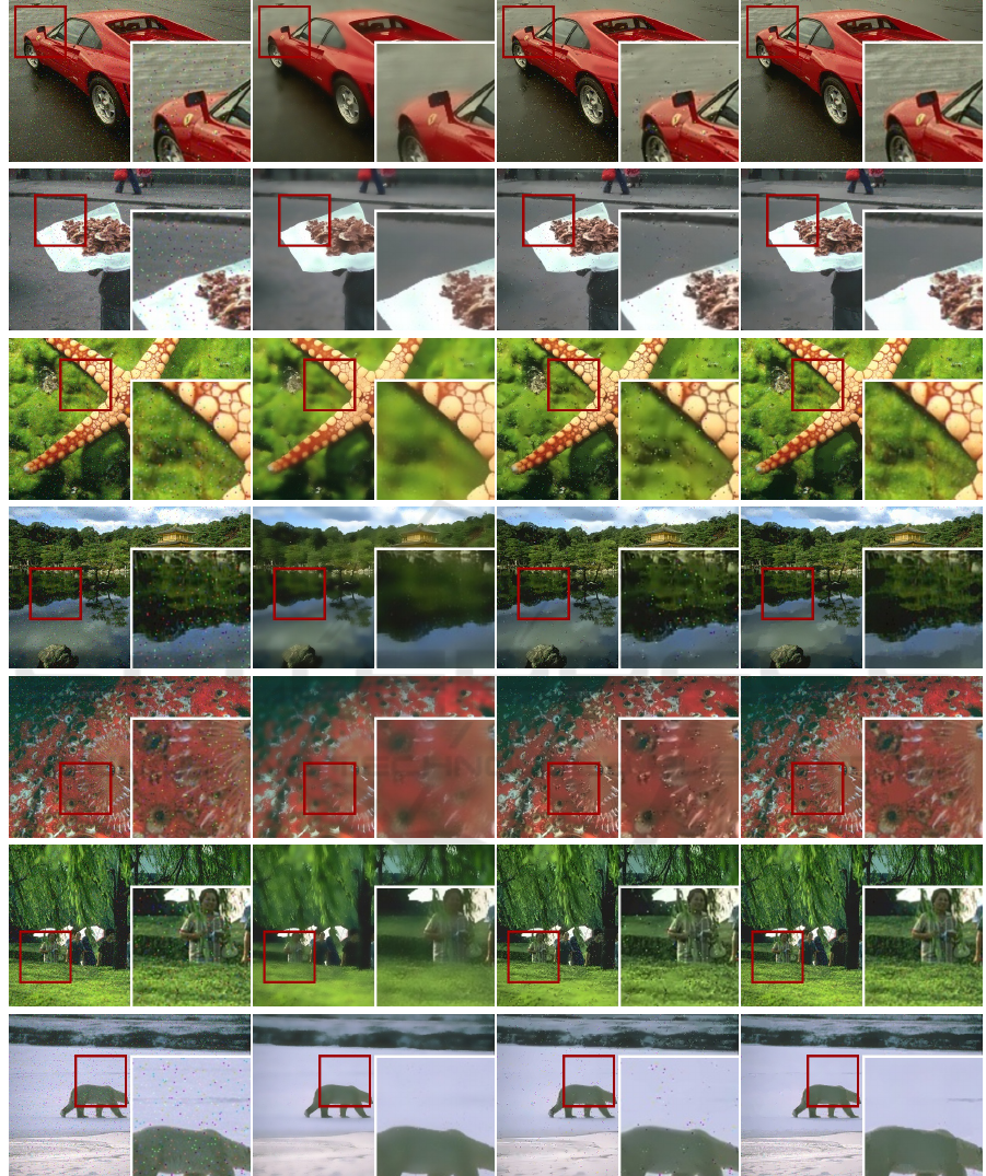
(a) Noisy test image. (b) Bilateral Filter. (c) Non-Local-Means Filter. (d) Proposed Filter.
Figure 7: Visual comparison of filter results. Quantitative results are shown in Tab. 1. Images taken from Berkeley Image
Dataset (Arbelaez et al., 2011).
This means, our system performs only slightly
worse than recent denoising methods, but offers real-
time performance, which makes the filter applicable to
video streams and hence can be used in the future as a
component inside the perception-action loop of robo-
tic applications. It enables image processing and data
VISAPP 2018 - International Conference on Computer Vision Theory and Applications
92

Table 2: Comparison of RMSE and PSNR computed on three different scenes: 1) an alternating line, 2) a sawtooth wave, and
3) a sinusoidal wave. To each scene three different noises (Gaussian (G.), salt-and-pepper (s&p), or both) is added, resulting in
9 different experiments. Each experiment is repeated 1000 times and averaged.
Gauss s&p Gauss and s&p
RMSE PSNR RMSE PSNR RMSE PSNR
1) Alternating Line
No denoising 10.0 22.3 15.2 16.4 18.1 17.2
EPF 2
2
2.
.
.6
6
6 3
3
32
2
2.
.
.3
3
3 3
3
3.
.
.9
9
9 2
2
28
8
8.
.
.5
5
5 5
5
5.
.
.1
1
1 2
2
26
6
6.
.
.7
7
7
Bilateral 6.9 25.3 15.2 16.4 16.5 17.7
Gaussian 6.0 25.3 7.8 22.2 8.7 22.1
Median 5.1 26.8 4.1 27.9 6.0 25.4
2) Sawtooth Wave
No denoising 10.0 21.6 14.1 17.1 17.1 17.0
EPF 3
3
3.
.
.7
7
7 2
2
29
9
9.
.
.3
3
3 4
4
4.
.
.6
6
6 2
2
26
6
6.
.
.5
5
5 6
6
6.
.
.6
6
6 2
2
24
4
4.
.
.5
5
5
Bilateral 7.0 24.4 14.0 17.1 15.5 17.5
Gaussian 7.6 22.6 8.8 20.9 9.6 20.6
Median 5.7 25.2 5.8 24.9 7.4 23.1
3) Sinusoidal Wave
No denoising 10.0 20.1 12.9 17.8 16.1 16.0
EPF 2
2
2.
.
.7
7
7 2
2
29
9
9.
.
.5
5
5 2.6 29.8 4
4
4.
.
.4
4
4 2
2
25
5
5.
.
.6
6
6
Bilateral 6.7 23.0 12.8 17.9 14.4 16.9
Gaussian 3.9 26.7 5.0 24.2 6.3 22.6
Median 4.1 26.1 0
0
0.
.
.6
6
6 4
4
46
6
6.
.
.1
1
1 4.5 25.6
Table 3: Time performance for images of different sizes. The
test images were taken from the validation set of the Berke-
ley Segmentation Dataset and Benchmark (Arbelaez et al.,
2011). 100 measurements were taken and averaged. Our
proposed EPF filter is compared to state-of-the-art algorithm
BM3D (Dabov et al., 2007) as shown in (Shao et al., 2014).
BM3D is, according to (Shao et al., 2014), one of the fastest
recent methods.
Image Size CPU GPU BM3D
[px] [Hz] [Hz] [Hz]
240 × 180 2.0 80.4
320 × 240 1.1 48.0
480 × 320 0.5 23.8 0.4
640 × 480 0.3 12.4
800 × 600 0.2 7.7 0.1
1024 × 768 0.1 4.2 0.1
Table 4: PSNR values for state-of-the-art methods (as shown
in (Gu et al., 2014)) compared to our proposed EPF filter.
Gaussian Noise Recent Methods EPF
σ = 10 33.5 − 34.8 30.7
σ = 30 27.8 − 29.2 23.0
σ = 50 25.1 − 26.8 19.9
σ = 100 21.6 − 23.6 15.5
filtering on embedded hardware, for example in flying
robots, which is another research area of ours. The
filter not only works well in the image domain, but can
be extended to data of any dimension, e.g. noisy 6d
point cloud data. In our work we demonstrated this by
filtering 1d sensor data. This work will be submitted
to the opencv image library (Bradski, 2000) to enable
easy usage and comparison to other methods.
ACKNOWLEDGEMENTS
The research leading to these results has received
funding from the European Communitys H2020 Pro-
gramme under grant agreement no. 680431, Recon-
Cell.
REFERENCES
Alvarez, L., Lions, P.-L., and Morel, J.-M. (1992). Image
selective smoothing and edge detection by nonlinear
diffusion. ii. SIAM Journal on numerical analysis,
29(3):845–866.
Arbelaez, P., Maire, M., Fowlkes, C., and Malik, J. (2011).
Contour detection and hierarchical image segmentation.
IEEE transactions on pattern analysis and machine
intelligence, 33(5):898–916.
Bradski, G. (2000). Opencv. Dr. Dobb’s Journal of Software
Tools.
Buades, A., Coll, B., and Morel, J.-M. (2005). A non-local
algorithm for image denoising. In IEEE Conference
on Computer Vision and Pattern Recognition(CVPR),
volume 2, pages 60–65. IEEE.
Dabov, K., Foi, A., Katkovnik, V., and Egiazarian, K. (2007).
Image denoising by sparse 3-d transform-domain col-
laborative filtering. IEEE Transactions on image pro-
cessing, 16(8):2080–2095.
A Real-Time Edge-Preserving Denoising Filter
93

Donoho, D. L. (1995). De-noising by soft-thresholding.
IEEE transactions on information theory, 41(3):613–
627.
Du, W., Tian, X., and Sun, Y. (2011). A dynamic threshold
edge-preserving smoothing segmentation algorithm for
anterior chamber oct images based on modified his-
togram. In 4th International Congress on Image and
Signal Processing (CISP), volume 2, pages 1123–1126.
IEEE.
Gonzalez, R. C. and Woods, R. E. (2002). Digital image
processing. Pearson Prentice Hall.
Gu, S., Zhang, L., Zuo, W., and Feng, X. (2014). Weighted
nuclear norm minimization with application to image
denoising. In Proceedings of the IEEE Conference
on Computer Vision and Pattern Recognition, pages
2862–2869.
Lev, A., Zucker, S. W., and Rosenfeld, A. (1977). Iterative
enhancemnent of noisy images. IEEE Transactions on
Systems, Man, and Cybernetics, 7(6):435–442.
Lin, T.-Y., Maire, M., Belongie, S., Hays, J., Perona, P.,
Ramanan, D., Doll
´
ar, P., and Zitnick, C. L. (2014).
Microsoft coco: Common objects in context. In Euro-
pean Conference on Computer Vision, pages 740–755.
Springer.
Lindenbaum, M., Fischer, M., and Bruckstein, A. (1994). On
gabor’s contribution to image enhancement. Pattern
Recognition, 27(1):1–8.
Mairal, J., Bach, F., Ponce, J., Sapiro, G., and Zisserman, A.
(2009). Non-local sparse models for image restoration.
In IEEE 12th International Conference on Computer
Vision, pages 2272–2279. IEEE.
Muneyasu, M., Maeda, T., Yako, T., and Hinamoto, T.
(1995). A realization of edge-preserving smoothing
filters using layered neural networks. In IEEE Inter-
national Conference on Neural Networks, volume 4,
pages 1903–1906. IEEE.
Pandey, M., Bhatia, M., and Bansal, A. (2016). An ana-
tomization of noise removal techniques on medical
images. In International Conference on Innovation
and Challenges in Cyber Security (ICICCS-INBUSH),
pages 224–229.
Perona, P. and Malik, J. (1990). Scale-space and edge
detection using anisotropic diffusion. IEEE Tran-
sactions on pattern analysis and machine intelligence,
12(7):629–639.
Reich, S., Abramov, A., Papon, J., W
¨
org
¨
otter, F., and Dellen,
B. (2013). A novel real-time edge-preserving smoo-
thing filter. In International Conference on Computer
Vision Theory and Applications, pages 5 – 14.
Rudin, L. I., Osher, S., and Fatemi, E. (1992). Nonlinear
total variation based noise removal algorithms. Physica
D: Nonlinear Phenomena, 60(1):259–268.
Shao, L., Yan, R., Li, X., and Liu, Y. (2014). From heuristic
optimization to dictionary learning: A review and com-
prehensive comparison of image denoising algorithms.
IEEE Transactions on Cybernetics, 44(7):1001–1013.
Sonka, M., Hlavac, V., and Boyle, R. (2014). Image proces-
sing, analysis, and machine vision. Cengage Learning.
Tomasi, C. and Manduchi, R. (1998). Bilateral filtering for
gray and color images. In Sixth International Confe-
rence on Computer Vision, pages 839–846. IEEE.
Yang, Q., Wang, S., and Ahuja, N. (2010). Svm for edge-
preserving filtering. In IEEE Conference on Computer
Vision and Pattern Recognition (CVPR), pages 1775–
1782. IEEE.
Zoran, D. and Weiss, Y. (2011). From learning models of
natural image patches to whole image restoration. In
IEEE International Conference on Computer Vision
(ICCV), pages 479–486. IEEE.
VISAPP 2018 - International Conference on Computer Vision Theory and Applications
94