
Accelerated Simulation of Brittle Objects for Interactive Applications
Philippe Meseure
1
, Xavier Skapin
1
, Emmanuelle Darles
1
and Guilhem Delaitre
2
1
University of Poitiers, CNRS, XLIM Lab, UMR 7252, 86962 Futuroscope CEDEX, France
2
University of Limoges, CNRS, XLIM Lab, UMR 7252, 87000 Limoges, France
Keywords:
Physically-based Animation, Fractures, Connected-component Detection, Topological Models, Real-time
Simulation.
Abstract:
This article presents a model that aims at computing deformation and simulating fractures. To allow the use
of linear elasticity in small displacements for deformation of a brittle object while still enabling any rigid
motion, a rigid reference is computed using the Shape Matching method and all displacements are evaluated
with respect to this reference. Fractures are handled using a stress tensor computed at each vertex of the
object’s 3D mesh. Some accelerations are proposed, that allow a faster determination of fracture areas and a
fast processing of new connected components.
1 INTRODUCTION
For a long time, fracture simulation has been one
of the main concerns of physically-based animation
(Terzopoulos and Fleisher, 1988; Norton et al., 1991).
However, despite the amount of proposed solutions,
it remains a tedious process. As far as “rigid” brit-
tle objects are concerned, the fracture simulation con-
sists in computing the (infinitesimal) deformation of
the object when subject to external constraints and
detecting where a local strain or stress exceeds some
threshold. Finite element models using linear elas-
ticity (Hooke’s constitutive law) has been proposed
in the pioneering work presented in (O’Brien and
Hodgins, 1999). However, such an approach and all
its derivatives require the (non-linearized) Green/St-
Venant deformation tensor which makes them more
computationally demanding. Real time finite element
methods usually assume that displacements are small
and use Cauchy’s infinitesimal strain tensor (Cotin
et al., 1999; Cotin et al., 2000). Since, in rigid bod-
ies, fractures occur upon small deformations, this ten-
sor seems a good choice for the simulation of such
objects. Unfortunately, it does not allow the object
to rotate (it produces large deformation instead), and
rigid displacements cannot directly be taken into ac-
count. This limit is crippling for rigid object simula-
tion. In this article, we propose a model that allows
both rigid motion computation and strain computation
using Cauchy’s linear tensor, which makes it well-
adapted for interactive or real time environments.
In time-critical applications, the fracture process
appears as a heavy step of the simulation that should
benefit from any solution that allows computation
time gains. We therefore highlight a method that
avoids the computation of a costly fracture criterion
by ignoring places where no fracture is likely to occur.
Moreover, since our method explicitly computes rigid
motion, it is necessary to handle each connected com-
ponent of the object separately. However, after a frac-
ture, a simulated object can split into multiple compo-
nents. Unfortunately, connected component detection
is a global topological property that requires a walk
through the whole mesh of the object. Ideally, this
walk should be proceeded only when new connected
component have actually appeared. We thus propose
the use of an oracle that avoids, as much as possible,
such a walk.
The paper is organized as follows: After the pre-
sentation of previous work in Section 2, the model
is detailed in Section 3. Section 4 presents how frac-
tures are handled and different process improvements.
Finally, Section 5 shows the obtained results before
concluding.
2 PREVIOUS WORK
Fracture simulation relies primarily on deformation
computation (Nealen et al., 2006), but many ap-
proaches exist (Muguercia et al., 2014). Indeed, when
a deformation is computed, different criteria can be
used to make cracks appear in the structure. Geomet-
ric criteria have been proposed, such as an elongation
28
Meseure, P., Skapin, X., Darles, E. and Delaitre, G.
Accelerated Simulation of Brittle Objects for Interactive Applications.
DOI: 10.5220/0006526400280039
In Proceedings of the 13th International Joint Conference on Computer Vision, Imaging and Computer Graphics Theory and Applications (VISIGRAPP 2018) - Volume 1: GRAPP, pages
28-39
ISBN: 978-989-758-287-5
Copyright © 2018 by SCITEPRESS – Science and Technology Publications, Lda. All rights reserved

of springs beyond a given threshold (Norton et al.,
1991) or an excessive strain tensor value (Terzopou-
los and Fleisher, 1988). Force or stress thresholds can
be used as well. Thus, O’Brien and Hodgins proposed
a simulation of fracture based on linear elasticity and
the computation of a separation tensor at each mesh
vertex (O’Brien and Hodgins, 1999). The separation
tensor of a vertex is obtained from the stress tensor
of the surrounding elements. By considering posi-
tive and negative eigenvalues separately, each tensor
is separated into a tensile tensor and a compressive
one. Tensor components of volumes surrounding a
node are associated to create a new node tensor that
allows to take into account both tensile and compres-
sive stresses. This method has been extended in var-
ious approaches, for instance (Pfaff et al., 2014) to
simulate 2D tearing and (Koschier et al., 2014) for
adaptive resolution models. To handle fractures, it is
also possible to rely on modal analysis (Glondu et al.,
2012), but this is a global method that can be quite
costly, especially for high resolution meshes. Bound-
ary element method have also been used (Hahn and
Wojtan, 2015; Hahn and Wojtan, 2016). Fractures
can also be applied on meshless models (Pauly et al.,
2005).
Cracks may be applied wherever a fracture crite-
rion is verified. However, it is possible to focus only
on high stress areas, and control cracks to avoid a
shattering effect (Koschier et al., 2014). Local ge-
ometry is not necessarily adapted to the topological
modifications that the mesh should undergo. Some
methods propose to virtually cut volumes while keep-
ing well-shaped elements but the used mesh is no
longer manifold (Molino et al., 2004). XFEM ap-
proaches consider discontinuous element shape func-
tions to represent and simulate fractures (Koschier
et al., 2017). Some interactive methods tend to
use predefined crack patterns that locally modify the
mesh (M
¨
uller et al., 2013; Chen et al., 2014; Parker
and O’Brien, 2009), but cracks are not “physically-
managed” in such cases. The solution proposed in
(Schvartzman and Otaduy, 2014) appears as a com-
promise where the crack pattern is completely applied
at the time of impact (no crack propagation) but is
adapted to the deformation energy field in the fractur-
ing body and can be user-controlled.
Different deformable models can be used to find
fracture zones, but many approaches rely on continu-
ous mechanics, solved by a finite element method, as
in (O’Brien and Hodgins, 1999) and subsequent work.
Since an object can break due to small displacements,
using a linearized, more computationally-efficient,
strain tensor is possible, but is not compatible with
rotations of the object. The corotational method con-
sists in computing local rotations at each node to ex-
tract rotation and focus on deformation only (M
¨
uller
et al., 2002). This method has been used to simu-
late fractures (M
¨
uller et al., 2004; Chen et al., 2014),
but is known to produce ghost forces. To avoid such
forces, a rotation can be computed, not for every node
but for every element. However, in such a case, the
fracture criterion should rely on the stress computed
for each element (M
¨
uller and Gross, 2004) and not on
each node. Indeed, a node has several possibly differ-
ent displacements, one for each surrounding element.
Considering a node-based measure of stress can be
seen as non-consistent. Approaches based on node
stress criteria for corotational FEM models have been
used in some work (Busaryev et al., 2013) although
they lack theoretical backgrounds.
To conciliate computationally-efficient deforma-
tion measures and rigid motions, some methods con-
sider that a brittle object deforms and eventually
breaks only for given situations. They propose to sim-
ulate this object as a perfectly rigid one, but switch to
a static computation of (linear) deformation in case of
collisions (M
¨
uller et al., 2001; Bao et al., 2007; Liu
et al., 2011). It is also the case in (Zhu et al., 2015)
by relying only on a surface mesh to compute both
deformation and crack path. Such approaches sup-
pose that only an instantaneous impact can produce
fractures. Nevertheless, to simulate a fracture result-
ing from a progressive deformation (see Figure 7), a
dynamic approach should be preferred (Glondu et al.,
2012; Koschier et al., 2014). Anyway, the simula-
tion of a rigid body simulation (with only 6 degrees of
freedom) is several orders of magnitude faster to com-
pute than a finite element mesh. In time-critical ap-
plications, the computation time of a simulation step
should be kept as constant as possible. It cannot be
envisaged to switch from a rigid body to a finite ele-
ment model without expecting a high variation of the
latency of the simulation system. Instead, for such ap-
plications, we think that simulating a breakable rigid
body, at every time step and not only time step with
collisions, using a low-deformable model is accept-
able.
Indeed, finite element methods for small displace-
ments appear to be fast enough to allow real-time in-
teractions (Cotin et al., 2000; M
¨
uller et al., 2002). To
deal with rotations, rigid motions should be computed
by an additional, coupled, model. The pioneering
work in (Terzopoulos and Witkin, 1988) has shown
how to combine rigid body laws of motion with lin-
ear deformations. Unfortunately, the equations of
rigid motion and deformation are coupled and there-
fore hard to solve in real time. The Shape Matching
method aims at finding the minimum deformation be-
Accelerated Simulation of Brittle Objects for Interactive Applications
29
tween a given shape and a modification of this shape.
This method has been used in Computer Graphics
to simulate the deformation of a body by comparing
the position of each node to its corresponding refer-
ence node in the undeformed body and adding a force
which tends to minimize the difference (M
¨
uller et al.,
2005). In practice, this approach consists in inserting
a spring between these two positions. The resulting
simulation is fast and allows some special animation
effects, but is usually not realistic. Note that, while
observing a moving deformable object, the separa-
tion between the rigid motion and the deformation of
the body is quite arbitrary. Shape Matching appears
as a way to define, by minimizing deformation, the
rigid reference component. This can appear as a non-
physical approach, since the motion of this rigid com-
ponent is not guaranteed to be continuous (motion is
not taken into account in the computation, only po-
sitions are relevant with this method). However, it is
possible to smooth the motion of the rigid component
to make it look like continuous. Shape Matching must
be applied separately for each connected component
of the object. More generally, any method that com-
putes rigid motions explicitly, should precisely detect
each new detected component after a fracture (M
¨
uller
et al., 2001).
To overcome the above-mentioned limitations,
this paper presents an approach that:
• Relies on linear elasticity to compute the deforma-
tion of a brittle object. Displacements are guar-
anteed to be small by optimizing the position of
a rigid reference from which displacements are
computed.
• Uses an accelerating technique based on Ger-
schgorin’s theorem to find fracture locations
rapidly.
• Uses an oracle based on “vertex splitting” to de-
tect the appearance of any new connected compo-
nent and update the computation of the rigid ref-
erence of each connected component.
3 AN ALMOST-RIGID
DEFORMABLE MODEL
In our model, the deformation is considered to be as
small as possible (remember that most brittle objects
appear to be rigid at the macroscopic scale). In other
words, most energy of the system should be spent
for rigid motion, while the remaining energy should
be used for deformation. At each time step, position
and orientation corresponding to the rigid motion are
both determined using the Shape Matching method
and allow to define a, so-called, “rigid reference”. In
(M
¨
uller et al., 2005), the Shape Matching method was
mainly used to avoid the use of a mesh, by supplying
a mass/spring model with a fast way to handle its vol-
umetric behavior. On the contrary, in our approach,
the Shape Matching aims at computing the position
and orientation of a rigid reference to compute a min-
imum deformation and maintaining, as long as pos-
sible, the hypothesis of small displacements required
by the linear elasticity continuous model.
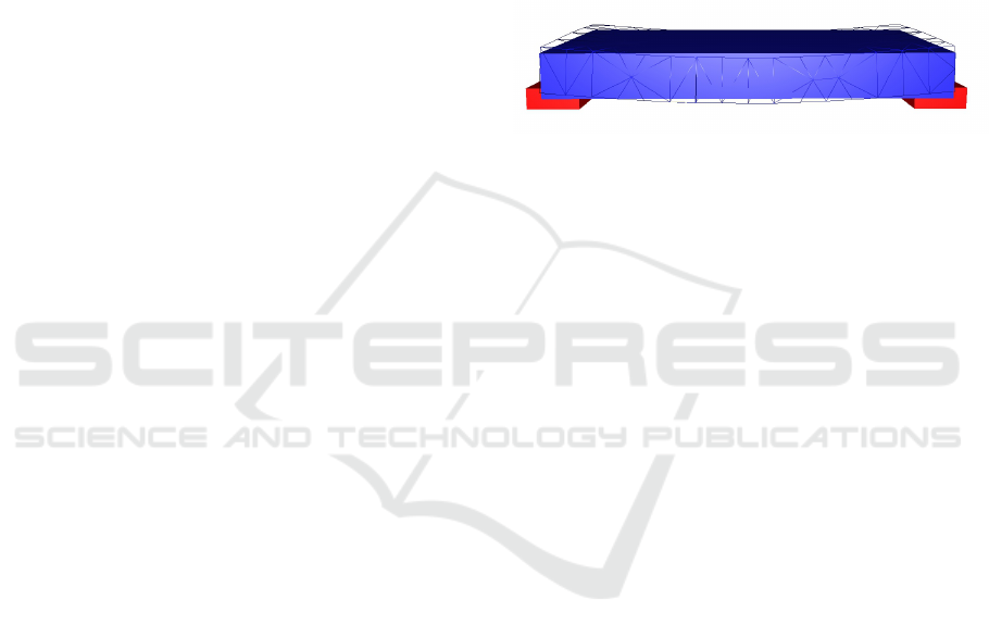
Figure 1 shows, for a block supported by immov-
able obstacles placed at its ends, both its deformed
state and rigid reference.
Figure 1: Model/reference coupling: A deformable model
(wireframe) is computed using dynamics laws and a rigid
reference (filled faces) is computed using Shape Matching.
3.1 Principles
Our model is a tetrahedral mesh where each vertex
i is characterized by a current position x
i
and a rest
position x
0
i
(defined in an undeformed and centered
configuration). At each time step, the process consists
in:
1. Applying Shape Matching with the current and
rest positions of the mesh vertices to obtain both
position (a translation vector τ) and orientation (a
rotation matrix R) of the rigid reference,
2. For each vertex, computing the reference position
x
ref
i
= Rx
0
i
+ τ and its displacements as d
i
= x
i
−
x
ref
i
,
3. Calculating the forces applied to each vertex by
each tetrahedron, using an explicit finite element
approach,
4. Summing all the forces applied to vertices, in-
ferring their accelerations and integrating them
twice,
5. Handling fractures.
An explicit finite element method is used (M
¨
uller
et al., 2001) to solve the equations of linear elastic-
ity based on Cauchy’s infinitesimal strain tensor. Let
C be the 6 × 6 stress-strain matrix based on Young
modulus and Poisson coefficient. For each tetrahe-
dron (e), both 6 × 12 strain-displacement matrix B
(e)
and 12 × 12 rigidity matrix K
(e)
are computed during
a pre-processing phase:
K
(e)
= B
(e)
T
CB
(e)
(1)
GRAPP 2018 - International Conference on Computer Graphics Theory and Applications
30

At each time step and for each tetrahedron (e), the
forces exerted on its vertices are computed as:
f
(e)
= K
(e)
d
(e)
(2)
where d
(e)
is a vector that gathers the displace-
ments of the four vertices, and f
(e)
gathers the forces
resulting from the deformation of the tetrahedron and
applied on the vertices.
The use of explicit or semi-implicit integration
schemes is theoretically possible, but in the case
of fractures, very small time step (microseconds or
tenths of microseconds) should be chosen. Indeed, to
simulate fracture and avoid large deformation, a high
stiffness (i.e. Young modulus) is required which di-
rectly impacts stability. Such small time steps are not
compatible with interactivity time constraints. The
implicit Euler method combined with the Newton-
Raphson method to solve non linear systems (Baraff
and Witkin, 1998) allows large time steps but can re-
sult in a highly-damped behavior for stiff systems.
Recently, exponential methods have been proposed
(Michels et al., 2017). These approaches allow the
resolution of stiff equations in a fast and robust way
while not loosing as much mechanical energy as im-
plicit methods. In our case, the implicit Euler system
is solved as proposed in (Hilde et al., 2001). This
method is mainly dedicated to small time steps and
does not require the computation of the Jacobian ma-
trix of the system while still allowing a good control
of the convergence of the system resolution. Other
integration methods such as implicit or exponential
ones could be used, for more efficient computation
times for instance, but not with the intent of reducing
the time step.
Fractures are handled as in (Koschier et al., 2014).
Note that after one or more fractures, multiple con-
nected components may appear. Shape Matching
must therefore be applied on each connected compo-
nent (R and τ are computed for each one), so a pre-
cise detection of any new component is mandatory. In
our implementation, all the vertices that belong to hte
same connected component share the same id. The
various simulation steps that depend on connected
components (for instance, the deformation computa-
tion) are slightly modified, to take into account the
data related to the concerned connected component,
using the id stored in vertices.
The overall algorithm for computing the behavior
of a body is given in algorithm 1.
3.2 Using Shape Matching
As explained in (M
¨
uller et al., 2005), for a given con-
nected component, the position of its rigid reference
Algorithm 1: computeDeformationForces().
Data: cc[] is a table containing the attributes of
each connected component
// Compute position and orientation
// of each connected component
computeCCState();
// Compute displacement of each vertex
foreach Vertex v do
Vec3 p = v.pos −cc[v.idCC].pos ;
Vec3 p0 = cc[v.idCC].orientation
T
× p ;
v.displacement = p0 − v.pos0 ;
end
// Compute deformation forces of each
// tetrahedron and distribute them
foreach Tetrahedron t do
Vec12 d = getVertexDisplacements(t) ;
Vec12 f = t.matK × d ;
foreach Vertex v of t do
v.force+ =
cc[v.idCC].orientation × f[v] ;
end
end
is defined as the position of the center of mass G of
its point cloud:
x
G
=
∑
N
i=1
m
i
x
i
∑
N
i=1
m
i
(3)
where N is the number of vertices in the mesh, m
i
the mass of each of them and x
i
their position. The
rotation is extracted from the following matrix:
A =
N
∑
i=1
p
i
x
0
i
T
(4)
where p
i
is the relative position of the i
th
vertex
with respect to the center of mass, that is p
i
= x
i
−x
G
.
The computation is shown in algorithm 2. Note that
there is no loop such as “for each element of a con-
nected component”, which could cause computation
time overheads due to dedicated walk through the
topological structure of the simulated body.
This method is basically an approach that com-
putes a position that minimizes the length of all p
i
(grouped in a single energy function). Unfortunately,
the method ignores the history of motion. Therefore,
the temporal continuity of the rigid reference’s ori-
entation cannot be ensured. In practice, when the
number of vertices is high enough, no discontinuity
is observed. Indeed, the global minimum of the en-
ergy function varies slightly. Nevertheless, orienta-
tion discontinuities may appear with regards to con-
nected components with a small number of vertices.
Accelerated Simulation of Brittle Objects for Interactive Applications
31

Algorithm 2: computeCCState().
foreach Vertex v do
// Accumulate position and mass
// into v’s connected component
cc[v.idCC].pos+ = v.pos ;
cc[v.idCC].mass+ = v.mass ;
end
// Compute positions
foreach Connected Component idCC do
cc[idCC].pos/ = cc[idCC ].mass ;
// Compute matrix of equation (4)
foreach Vertex v do
p = v.pos − cc[v.idCC].pos ;
cc[idCC].matA+ = p × v.pos0
T
;
end
// Compute orientations
foreach Connected Component idCC do
cc[idCC].orientation =
extractRotation(cc[idCC].matA) ;
In this case, several local minima exist, and the global
one rapidly changes among these.
It turns out that only isolated tetrahedra (in other
words, connected components with only four ver-
tices), exhibit such a discontinuous behavior. We have
investigated a first solution that considers isolated
tetrahedra as rigid, since they are atomic elements of
the initial mesh. This can be done in our algorithm
using only a slight modification, by considering that
rigid bodies can be simulated using a constrained de-
formable model (van Overveld and Barenbrug, 1995).
More precisely, the vertices are first moved according
to external forces, then Shape Matching is computed
for the tetrahedron, as done for any connected com-
ponent of the model. After that step, current vertex
positions x
i
in isolated tetrahedra are projected onto
their corresponding reference position (x
ref
i
). Veloc-
ity is adapted accordingly. This solution has a draw-
back: Isolated pseudo-rigid tetrahedra tend to stop ro-
tating quite quickly. Indeed, angular momenta are not
explicitly maintained by this approach, rotations re-
sult from the difference of velocities of the vertices
of the tetrahedra. Since vertices are forced to keep
their tetrahedron undeformed, they tend to loose ve-
locity and therefore, the orientation of their tetrahe-
dron steadies rapidly.
We have investigated another solution to compute
rotation of isolated tetrahedra, by using a QR decom-
position as proposed in (Nesme et al., 2005). This
method provides better stability for tetrahedra (i.e. ro-
tation matrix continuity), provided that the QR de-
composition is handled with the same vertex order be-
tween two steps.
3.3 Display
Even if a high Young modulus is applied, the object
can still exhibit visible deformations due to the com-
putation time step which is too large for fractures (see
Figure 1). To guarantee an accurate display of the ob-
ject, the rigid reference can be displayed instead of
the deformable body itself. This approach works well
in practice, but has an impact on the collision process
of the simulation, if overlaps must be avoided. For-
tunately, since the reference body is not physically
simulated, any modification of position and orienta-
tion can be applied arbitrarily, for display only. Any
correction method that controls the position and ori-
entation of a rigid body, such as an optimization algo-
rithm to minimize overlap, can therefore be applied.
In our simulation, no correction was however neces-
sary, since overlaps were low enough in practice.
Shape Matching is applied independently on each
connected component. Should a new connected com-
ponent appear after a fracture, it is unlikely that its
newly-computed position and orientation are contin-
uous with respect to the position and orientation it
had previously, when it was still connected. Fig-
ure 2 illustrates this discontinuity problem. To avoid
the discontinuity of display, an interpolation between
its previous state and its newly-computed one is ap-
plied. More precisely, a current state is first com-
puted, based on its original connected component.
This can be easily made by applying Shape Matching
on
x
ref
i
positions. Next, a target state is computed
by applying Shape Matching on
{
x
i
}
positions. Af-
ter a fracture, current and target states differ. Target
state should be used for the display of its correspond-
ing connected component, but its position may be too
far from the position where it was previously located.
Current state corresponds to the location of the con-
nected component at the fracture time. During the
following time steps, we choose to modify the posi-
tion and orientation of the current state so that it tends
to reach the target state. Although a proportional-
derivative controller could be used for this purpose,
only a simple proportional controller has been used
in our implementation and gives satisfying results in
practice. Let τ
cur
and τ
target
be the current and the
target translations respectively. Then τ
cur
is updated
to τ
cur
+ α(τ
target
− τ
cur
), where α is a small value
(typically 0.1 or less). A similar approach is used
for rotation, based on quaternions, since they offer
a convenient way to interpolate rotations (Shoemake,
1985). If q is a quaternion representing the rotation
that transforms the current orientation into the target
orientation of a connected component, the quaternion
q + 1 represents (after renormalization) half this rota-
tion. By repeating this simple formula several times,
GRAPP 2018 - International Conference on Computer Graphics Theory and Applications
32
we can quickly divide the angle of rotation between
current and target orientation by any power of 2. Ac-
cordingly, the α value used for translation is chosen
as the corresponding negative power of 2.
Note that the target state is also updated at each
time step, since all x
i
positions change. A more gen-
eral approach, where a rigid reference is simulated as
a perfect rigid body, linked by two springs, one linear
and the other one angular, to the deformed configu-
ration, and subject to collisions constraints is another
way to compute the current state at each time step.
This approach is physically-based but results in a 2
nd
-
order control of the current state used for display, so
possibly an undesirable latency.
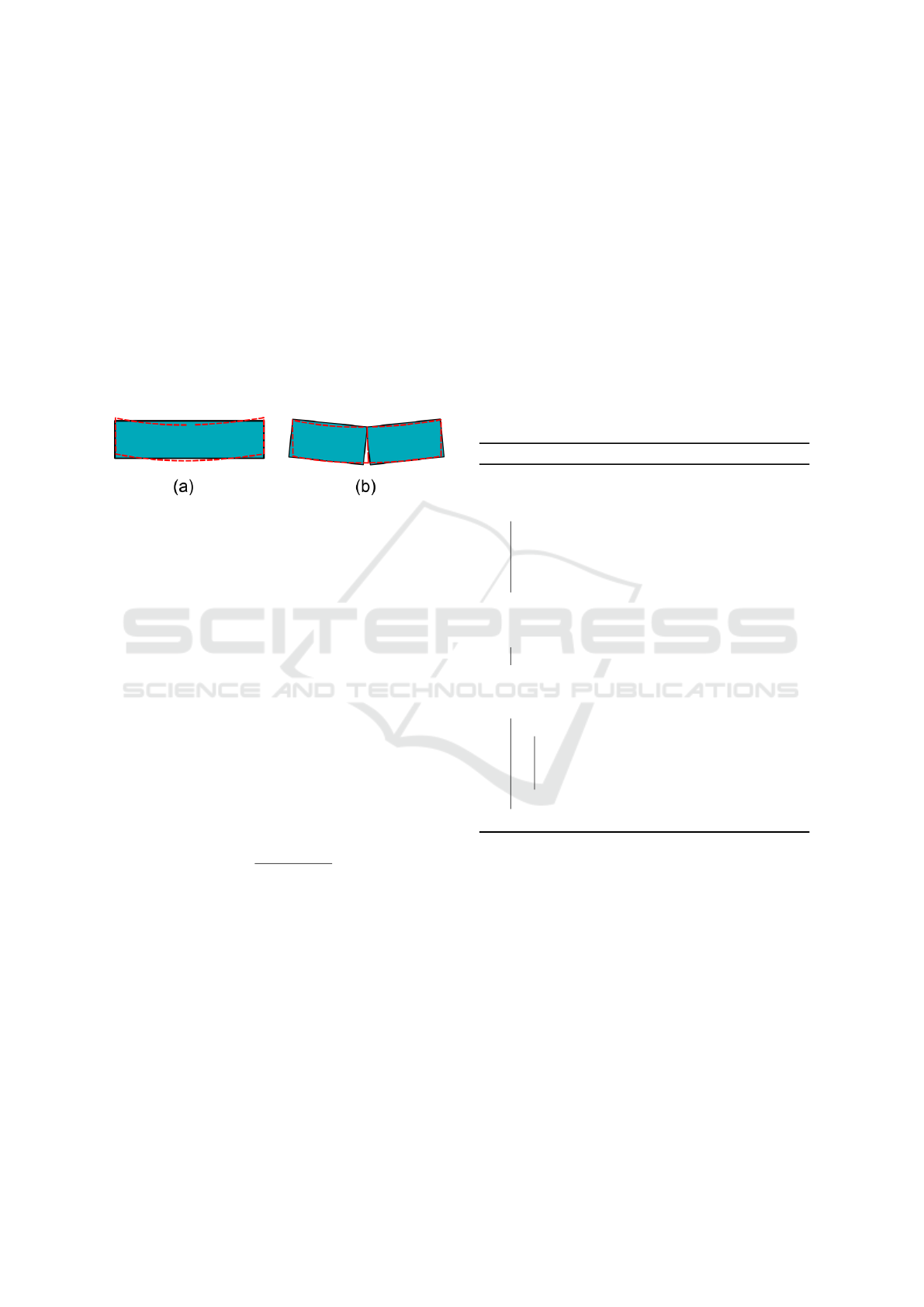
Figure 2: Discontinuity issue with Shape Matching. (a) A
red block is deformed (red dotted line) and Shape Matching
provides a position of the rigid reference (solid line). (b)
A fracture occurs and the object is split. Shape Matching
is separately applied on both connected components and re-
sults in a discontinuous state with respect to their positions
in (a).
4 FRACTURE PROCESS
Due to the linear interpolation functions used by the
finite element method, the stress tensor is constant all
over each tetrahedron and can be computed as:
σ
(e)
= CB
(e)
d
(e)
(5)
As proposed in (Koschier et al., 2014), a node
stress tensor can be computed for each vertex as:
σ =
∑
(e)
m
(e)
σ
(e)
∑
(e)
m
(e)
(6)
where m
(e)
is the mass of the element (e). Here,
the expression has been slightly modified compared
to the original article, but the result is the same. Our
notation only aims at showing that it is basically a
weighted average value of surrounding element stress
tensors. Note that, if each tetrahedron provides each
of its vertices with a quarter of its mass (mass lump-
ing technique), the denominator of equation 6 corre-
sponds to the mass of the concerned node multiplied
by 4. A fracture is applied on some vertex when
at least one eigenvalue of its stress tensor exceeds a
given threshold ξ. A fracture plane is built using the
related eigenvector as its normal. Each surrounding
tetrahedron is marked as “positive” or “negative” de-
pending on the side of the plane where its center is po-
sitioned. Any face that is adjacent to a pair of tetrahe-
dra with different signs is split to separate them. The
whole process aims at splitting a fan of faces around
the “fracture vertex” to make it split. If a fracture gen-
erates new connected components, these components
must be identified to allow distinct Shape Matching
applications when needed. This represents the last
step of the fracture process.
To accelerate this process, two lines of approach
have been considered: a fast location of fracture zones
and a fast identification of new connected compo-
nents. The algorithm 3 give an overview of the frac-
ture process.
Algorithm 3: findFractures().
// Compute each tetrahedron stress tensor
and report it to its vertices
foreach Tetrahedron t do
Vec12 d = getVertexDisplacements(t) ;
t.σ = matC ×t.matB × d ;
foreach Vertex v of t do
v.σ+ = t.mass ×t.σ ;
end
// Average each vertex stress tensor
foreach Vertex v do
v.σ/ = (4 × v.mass) ;
end
// Check where a fracture occurs
foreach Vertex v do
if gerschgorinTest(v.σ,ξ) then
Vec3 eigenval = eigenValues(v.σ) ;
if max(eigenval) ≥ ξ then
split(v,eigenvec(max(eigenval)) ;
end
end
4.1 Finding Fracture Location
One important time loss during fracture location
comes from the necessity to compute eigenvalues of
stress tensors, merely to determine if one of them may
exceed some threshold ξ. In mechanical engineering,
this step is often sped up using the Gerschgorin’s the-
orem which, to our knowledge, has never been pro-
posed to the Computer Graphics community. This
theorem states that an upper bound of the eigenvalues
of a square matrix M can be computed considering
the sum of absolute values of some of its terms. In our
case, M is a symmetric matrix, so the upper bound can
be found by computing the maximum value of three
Accelerated Simulation of Brittle Objects for Interactive Applications
33

terms b
i
, one for each column i:
b
i
= M
ii
+
∑
j6=i
M
ji
(7)
After calculating the stress tensor of a vertex, the
associated b
i
values are computed. If all of them re-
main below the fracture threshold, no fracture appears
at this vertex and the eigenvalues computation can be
avoided. On the contrary, if the test fails, the eigenval-
ues must be computed since, if at least one of them is
greater than the given threshold, its associated eigen-
vector must be known for the following steps. Note
that the overall complexity is small, since only 6 float-
ing point additions, 6 absolute values and 3 compar-
isons are necessary to complete Gerschgorin’s test at
a vertex.
4.2 Connected Component
Determination
Each connected component of the body is character-
ized by a rigid reference, defined as a current state
(position and orientation) and a target state. When
a fracture occurs, one or more new connected com-
ponents might appear, which should be clearly iden-
tified to update their states. Connected components
identification requires to scan all the elements (for in-
stance vertices) of the current connected component
and mark them (more precisely, in our implementa-
tion, “marking vertices” means providing them with
the id of their connected component). If some ele-
ments are not marked (i.e. these elements still store
the id of their connected component before fracture),
that means that another connected component must
be identified. Reversely, if all elements are marked,
that means that no other connected component exists.
This is a time-consuming process (linear with respect
to the number of elements to be marked, i.e. vertices
or volumes) that should be avoided when no new con-
nected component is created (in other words, when a
first walk would uselessly mark every element).
We propose to use an oracle that can test this case,
in order to speed up the overall component identifica-
tion. Of course, it must be efficient enough to avoid
false positive cases as much as possible (that is, cases
where the oracle announces new connected compo-
nents whereas no such component has appeared ac-
tually). Moreover, the oracle should be fast enough:
If its computation algorithm is too complex, it will
not be able to compete with a complete walk through
the structure. We found an efficient oracle by con-
sidering how many vertices split after each face split.
Indeed, when two adjacent tetrahedra are separated,
the support edges and vertices of the face must nec-
essarily split to allow the creation of a new connected
component. In Figure 3, it is shown that the three ver-
tices and three edges of a triangular face actually split
when a new connected component appears. Note that
if three vertices split, then the three edges necessar-
ily split. Therefore, after a face split, the vertices and
only the vertices of the face are checked for a split.
If, at least, one of these does not split, it is ensured
that no new connected component has been created.
On the contrary, if the three vertices split, then a new
connected component may appear, and this should be
checked further. Note that the vertex split criterion
must be checked after the split of each face of a fan
and not once the overall split is over. An appropriate
topological model should be used to ensure that the
vertex split is tested effectively (Lienhardt, 1994).
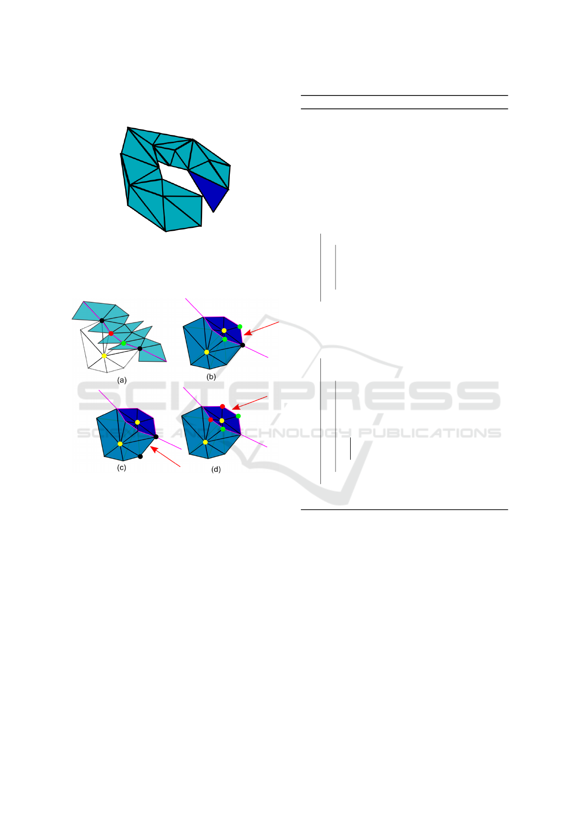
Figure 3: Oracle to detect if one new connected component
appears after a face split. In (a), only one vertex and two
edges split, so there is no new connected component. In (b),
three vertices and three edges split, so one new connected
component may appear.
Note that both criteria are local whereas the con-
nected property is global. It cannot be expected that
our oracle produces only right predictions, false pos-
itives are still possible: For instance, such a phe-
nomenon appears when two parts of an object are lo-
cally separated, but are still joined if the entire struc-
ture is considered, as shown in Figure 4. When using
the vertex split oracle, face ordering may sometimes
influence the final result and produce false positive
cases,as shown in Figure 5. For each subfigure, the
red arrow shows the last face that is split. In (a), only
two vertices (green and yellow) split and in (b), only
one vertex (yellow) splits. In such cases, the oracle is
right and states that there cannot be a new connected
component (which is the case: the surrounding parts
remain adjacent, for instance around the black ver-
tices, since these vertices do not split). In (c), how-
ever, the last face makes three vertices split (red, green
and yellow ones). In this case, the oracle is false,
since it concludes that a new connected component
has appeared. Note that, if only one other face re-
mained to be split at that time, the central vertex of
the fan would not split (it splits only when the last
face is split) and the oracle would not conclude that
a new connected component appears. As a conse-
quence, faces of fans with an edge at the surface of
the object (as it is the case in the figure) should be
checked first if possible, because these faces produces
GRAPP 2018 - International Conference on Computer Graphics Theory and Applications
34
false positive if split at the end of the process. The al-
gorithm 4 show the complete split process.
Figure 4: False positive of any local oracle. A local sep-
aration has occured, so any local oracle predicts a new
connected component, but the separated faces still belong
to the same connected component (initially topologically-
equivalent to a torus).
Figure 5: False positive of split vertex oracle. (a) represents
a series of adjacent edges (in magenta) at the mesh surface
(in blue). A fan (dotted lines) is defined around a vertex (in
yellow), inside the mesh, just below the surface faces. In
(b) and (c), if the pointed face is the last face to be split, at
least one of its vertex (in black) does not split. In (d), if the
pointed face is the last face to be split, the oracle predicts a
new connected component as its three vertices (red, yellow
and green) split. This face, with an edge at the surface of
the mesh, should be split when at least one other face of the
fan has not been split yet.
5 RESULTS
Several examples have been simulated and are repre-
sented in Figures 6 and 7. In both cases, the simu-
lated object is the same. The first one (Figure 6) cor-
responds to a classical fracture scenario where rigid
objects are shot toward a breakable one. This example
shows the shattering effect obtained when a fracture
Algorithm 4: split(v,u).
Data: v is a vertex
Data: u is the normal of the fracture plane
curidCC = v.iddCC ;
// Get the signs of tetrahedra around v
relatively to fracture plane
foreach Tetrahedron t around v do
t.sign = getSign(center(t), plane(v,u)) ;
// Search for faces adjacent to
// positive and negative tetrahedra
Bool newCC = f alse ;
foreach Face f around v do
if tetrahedra( f ) have different signs then
splitFace(f) ;
// Check for oracle
if all vertices( f ) have split then
newCC = true ;
end
end
// If oracle predicts new connected
components, identify them
if not newCC then return;
foreach Split Face f do
Vertex v1 =one of f ’s vertices ;
if v1.idCC == curidCC then
newidCC = getNewIdCC() ;
// Only loop over
// a connected component
foreach Vertex v2 in
connectedcomp(v1) do
v2.idCC = newidCC ;
cc[newidCC]+ = v2.mass ;
end
end
end
releaseIdCC (curidCC) ;
is applied wherever the fracture criterion is true. The
second case study (Figure 7) corresponds to a tension
that progressively deforms an object so that it eventu-
ally breaks. First, this example shows that fractures
may appear well after a collision has occurred, so the
dynamic approach of fracture is mandatory. Second,
it illustrates that the display of the rigid reference is
very useful. Indeed, in practice, the deformable mesh
undergoes visible deformations before fracturing (this
is the reason why the object does not break imme-
diately). The display of the deformable mesh would
not have produced the same visual effect. Another
case study aims at simulating a more complex object,
namely the Stanford Bunny (Figure 8). The mesh pa-
rameters used by the simulation are given in table 1.
In these scenarios, collision and self-collision de-
Accelerated Simulation of Brittle Objects for Interactive Applications
35
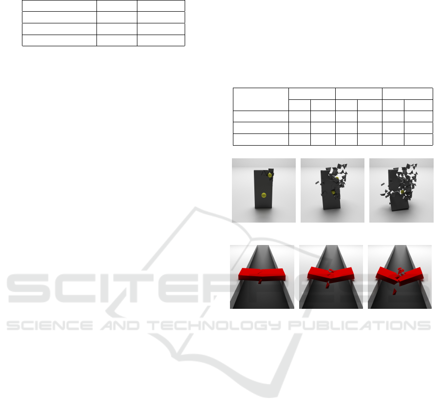
Table 1: Different test scenarios and their characteristics.
Scenarios #Tetras #Vertices
Struck monolith 413 174
Strained block 413 174
Falling bunny 6142 1363
tection has been handled using an approximative but
fast approach. They were mainly based on a penalty
method: Any environment obstacle is approximated
by a force field (for instance, ground or rigid bodies).
Every tetrahedron of the breakable body is bounded
by a sphere that also produces a repulsive force field
for points located inside it. Each vertex is checked
against all the force fields (a regular grid is used for
speeding up this step). Collision between vertices and
tetrahedron force fields are taken into account only if
they do not belong to the same connected component
(this is quickly determined as each vertices knows
the id of its connected component). A more precise
but efficient collision detection and response could be
used (Glondu et al., 2014), but requires to be adapted
to deformable bodies if used in our approach.
Note that the Broyden method to solve the implicit
integration equations does not converge as quickly
as a Newton-Raphson resolution. Note also that
no parallelization (CPU multithreading or GPU) has
been applied on the algorithms, except the use of
SIMD processor instructions for FEM computations.
We are completely aware that these times could be
largely improved as most similar approaches are usu-
ally based on GPU programming. However, the frac-
ture process is hard to parallelize in practice (because
of conflict access to the topological structures of the
object). This is why we did not worry on paralleliz-
ing the simulation itself to get a better performance
and chose to focus on fracture only.
The average and maximum simulation times are
shown in Table 2 for both corotational and our shape-
matching-based method. These times correspond to
a complete time step, including collision and self-
collision detection. The same object with the same
physical properties are simulated in both methods. As
shown, the corotational method is always slower than
ours. This mainly shows that the rotations for each
volume element always require more time to com-
pute than a shape-matching on the connected com-
ponents. Applying fractures on a simulated model
usually implies a computation time overhead, about
20% for simple models but that can be up to 50%
for the stanford bunny (which involves a lot of mul-
tiple synchroneous fractures). The maximum compu-
tation time when applying fractures is also mentioned
in the table, although we do find this time very sig-
nificant. Indeed, we have noticed that this maximum
time usually occurs once, at the beginning of a frac-
turing phase, and is not reached anymore during the
subsequent fractures.
Table 2: Average and maximum simulation times ob-
tained for our different scenarios using corotational and our
method without fracture (i.e. with an unreachable fracture
threshold). For our method, the average and maximum
computation times with fractures is also given. All these
times include collision and self-collision detection.
Scenarios Corotational Our method With fractures
av. max. av. max. av. max.
Struck monolith 34 60 28 44 34 84
Strained block 27 53 17 26 20 70
Falling bunny 291 408 218 380 340 1320
Figure 6: Two balls striking a monolith.
Figure 7: A brittle block collapses under its own weight.
The effect of the different accelerations have been
evaluated. First, the impact of Gerschgorin’s test
has been measured. This test is, in average, 3 times
faster than an immediate computation of the eigen-
values. Table 3 shows the effectiveness of this test,
since about 80% or more successful tests actually cor-
respond to a large eigenvalue that implies a fracture.
The split vertex oracle for new connected compo-
nents has also been tested. In table 3, the efficiency,
that is the ratio of true positives, for the split-vertex
oracle has been measured, in our different test cases.
It can be seen that, for over 90% of cases, the oracle
is right. So the oracle is a satisfactory way to detect
if some new component has appeared. Note also that,
in all our experiments, the oracle has never produced
any false negative.
Table 4 shows the computation times dedicated to
the fracture process. Several comments can be made.
First, the worst case for the basic rupture process, that,
by default, searches for new connected components,
occurs when no new connected component is created.
Indeed, all the structure must be (uselessly) walked
through to find this result. This proves that an ora-
cle that speeds up the new connected component de-
GRAPP 2018 - International Conference on Computer Graphics Theory and Applications
36

Table 3: Efficiency of Gerschgorin’s test and split-vertex oracle for different scenarios. The third column represents the
number of fan splits. The fourth column represents the number of fractures that actually result in the creation of new connected
components (CC) and the corresponding ratio. The fifth column represents the number of cases where the split-vertex oracle
predicts new connected components, the corresponding ratio, as well as the efficiency calculated by checking if new connected
components actually appeared.
Gerschgorin #fractures #CC creations #new CC predictions
Scenarios efficiency # ratio # ratio efficiency
Struck monolith 85% 198 112 56.6% 119 61.1% 94.1%
Strained block 92% 190 104 54.7% 111 58.4% 93.7%
Falling bunny 78% 1639 759 46.3% 833 50.8% 91.1%
tection is really of interest. Next, the additional cost
of using split-vertex oracle is measured by compar-
ing the computations times in case of new connected
component creation using the oracle or not. This cost
represents of at most 2% of computation time. But,
this cost is clearly justified, because, when no new
component appears, the rupture time can be reduced
by, at least, 55%, and the global reduction can reach
67%.
Table 4: Computation times for the rupture process in dif-
ferent scenarios with and without split-vertex oracle, for
ruptures that create new connected components (CC) or not.
Without Oracle (ms) With Oracle (ms)
Scenarios new CC no new CC new CC no new CC
Struck monolith 0.97 1.2 0.99 0.5
Strained block 0.96 1.06 0.98 0.48
Falling bunny 30.73 32.3 31.2 10.66
To provide a meaningful comparison, we have im-
plemented the same node tensor fracture criterion on
a corotational FEM (even if, in previous work sec-
tion, we pointed out that this approach was lacking
a theoretical background). This implementation also
uses the Gerschgorin’s theorem to speed up the broad-
phase that seeks for fracture nodes. We found that
corotational FEM tends to produce lower node stress
tensors (which is quite expected: Node displacements
are lower since element rotations are cancelled). As
a consequence, the shattering effect is reduced and
the final animation is quite different from the one ob-
tained with our method based on Shape Matching.
6 LIMITATIONS
The obtained fracture results heavily depend on
the initial tetrahedral mesh of the simulated object.
Remeshing techniques could be used to adapt the
mesh in the fracture zone, as several approaches have
already proposed (Su et al., 2009; M
¨
uller et al., 2013).
These techniques are compatible with our method,
provided that the rest positions and mass of the new
vertices that appear after a remeshing are determined
and the mechanical data of elements (stiffness and
strain/deformation matrices) are updated accordingly,
which can be done at the price of a little computation
time. These techniques apply on a given connected
component, so no side-effect on existing connected
components are expected during the remeshing.
We actually investigated a local remeshing solu-
tion based on tetrahedron subdivisions based on Loop
scheme as proposed in (Meseure et al., 2015). This
kind of remeshing is adapted to physical simulation
since the shape of most elements is preserved, al-
though scaled by a factor 1/2. This solution works
well in practice for deformable body simulation, how-
ever, it is not adapted to fracture. Indeed, after a sub-
division, the strain-displacement matrix B
(e)
of each
new elements is scaled by a factor 2 and its volume,
and consequently its mass, by a factor 1/8. The node
stress tensor (Equation 6) is directly impacted by such
modifications and the choice of mass as a weighting
coefficient is no longer adapted if the resolution of the
mesh is not uniform. Without a meaningful computa-
tion of node stress tensors, the criterion used to detect
fracture (a high eigenvalue) is no longer relevant. As
proposed in(Pfaff et al., 2014) in 2D, a more appro-
priate tensor, that is, independent on mesh resolution,
should be computed. More investigations are needed.
7 CONCLUSION AND FUTURE
WORK
This paper has presented a model that allows the
computation of small deformations of a brittle ob-
ject while still allowing rigid motions. To speed up
fracture management, the Gerschgorin’s test has been
proposed to easily locate fracture zones. A simple
oracle is also used to prevent the execution of heavy
algorithms needed in case of new connected compo-
nents. These improvements provide interesting com-
putation times, although no parallelization has been
exploited to compute deformations. It is definitely
one of our major goals, although the fracture pro-
Accelerated Simulation of Brittle Objects for Interactive Applications
37

cess itself is not really parallelizable. We also want
to improve visualization, by displaying more complex
fracture surfaces as done in (Koschier et al., 2014) (it
would only be a visual artifact, with no cost on the
fracture process itself). Furthermore, one remaining
problem concerns the number of cracks (that is fan
splitting) that can be handled in one step. Indeed,
if only one crack is allowed per simulation step, no
shattering effect occurs in general. The number of
handled cracks should however be bounded.
ACKNOWLEDGMENTS
We would like to thank the anonymous reviewers for
their comments that helped us to improve this paper.
This work has benefited from the financial support of
a M.Sc internship from the MIRES federation.
Figure 8: Shattering fracture of Stanford Bunny. The bot-
tom picture aims at highlighting the fracture surface and the
different connected components.
REFERENCES
Bao, Z., Hong, J.-M., Teran, J., and Fedkiw, R. (2007).
Fracturing rigid materials. IEEE Transactions on Vi-
sualization and Computer Graphics, 13(2):370–378.
Baraff, D. and Witkin, A. (1998). Large steps in cloth simu-
lation. In Proceedings of ACM SIGGRAPH 98, Com-
puter Graphics annual conference series, pages 43–54,
Orlando.
Busaryev, O., Dey, T. K., and Wang, H. (2013). Adaptive
fracture simulation of multi-layered thin plates. ACM
Transactions on Graphics (Proceedings of ACM SIG-
GRAPH 2013), 32(4).
Chen, Z., Yao, M., Feng, R., and Wang, H. (2014). Physics-
inspired adaptive fracture refinement. ACM Transac-
tions on Graphics (Proceedings of ACM SIGGRAPH
2014), 33(4).
Cotin, S., Delingette, H., and Ayache, N. (1999). Real-time
elastic deformations of soft tissues for surgery simu-
lation. IEEE Transactions on Visualization and Com-
puter Graphics, 5(1):62–73.
Cotin, S., Delingette, H., and Ayache, N. (2000). A hybrid
elastic model allowing real-time cutting, deformation
and force-feedback for surgery training and simula-
tion. The Visual Computer, 16(8):437–452.
Glondu, L., Marchal, M., and Dumont, G. (2012). Real-
time simulation of brittle fracture using modal anal-
ysis. IEEE Transactions on Visualization and Com-
puter Graphics, 19(2):201–209.
Glondu, L., Schvartzman, S. C., Marchal, M., Dumont, G.,
and Otaduy, M. A. (2014). Fast collision detection for
fracturing rigid bodies. IEEE Transactions on Visual-
ization and Computer Graphics, 20(1):30–41.
Hahn, D. and Wojtan, C. (2015). High-resolution brittle
fracture simulation with boundary elements. ACM
Transactions on Graphics (Proceedings of ACM SIG-
GRAPH 2015), 34(4).
Hahn, D. and Wojtan, C. (2016). Fast approximations for
boundary element based brittle fracture simulation.
ACM Transactions on Graphics (Proceedings of ACM
SIGGRAPH 2016), 35(4).
Hilde, L., Meseure, P., and Chaillou, C. (2001). A fast im-
plicit integration method for solving dynamic equa-
tions of movement. In Proceedings of the ACM Con-
ference on Virtual Reality Software and Technology,
pages 71–76, Banff.
Koschier, D., Bender, J., and Thuerey, N. (2017). Robust
extended finite elements for complex cutting of de-
formables. ACM Transactions on Graphics (Proceed-
ings of ACM SIGGRAPH 2017), 36(4).
Koschier, D., Lipponer, S., and Bender, J. (2014). Adap-
tive tetrahedral meshes for brittle fracture simulation.
In Proceedings of the ACM SIGGRAPH/Eurographics
Symposium on Computer Animation, pages 57–66,
Copenhagen.
Lienhardt, P. (1994). N-dimensional generalized combi-
natorial maps and cellular quasimanifolds. Int. J. of
Computational Geometry and Applications, 4(3):275–
324.
Liu, N., He, X., Li, S., and Wang, G. (2011). Meshless sim-
ulation of brittle fracture. Computer Animation and
Virtual Worlds, 22(2–3):115–124.
Meseure, P., Darles, E., Skapin, X., and Touileb, Y. (2015).
Adaptive resolution for topology modifications in
physically-based animation. Technical report, XLIM
lab.
Michels, D. L., Luan, V. T., and Tokman, M. (2017). A
stiffly accurate integrator for elastodynamic problems.
ACM Transactions on Graphics (Proceedings of ACM
SIGGRAPH 2017), 36(4).
Molino, N., Bao, Z., and Fedkiw, R. (2004). A virtual node
algorithm for changing mesh topology during simula-
tion. ACM Transactions on Graphics (Proceedings of
ACM SIGGRAPH 2004), 23(3):385–392.
Muguercia, L., Bosch, C., and Patown, G. (2014). Frac-
ture modeling in computer graphics. Computers and
Graphics, 45(C):86–100.
M
¨
uller, M., Chentanez, N., and Kim, T.-Y. (2013).
Real time dynamic fracture with volumetric approxi-
mate convex decompositions. ACM Transactions on
Graphics (Proceedings of ACM SIGGRAPH 2013),
32(4).
GRAPP 2018 - International Conference on Computer Graphics Theory and Applications
38

M
¨
uller, M., Dorsey, J., McMillan, L., Jagnow, R., and Cut-
ler, B. (2002). Stable real-time deformations. In Pro-
ceedings of the ACM SIGGRAPH/Eurographics Sym-
posium on Computer Animation, pages 49–54, San
Antonio.
M
¨
uller, M. and Gross, M. (2004). Interactive virtual mate-
rials. In Graphics Interface, pages 239–246, London
(Canada).
M
¨
uller, M., Heidelberger, B., Teschner, M., and Gross, M.
(2005). Meshless deformations based on shape match-
ing. ACM Transactions on Graphics (Proceedings of
ACM SIGGRAPH 2005), 24(3):471–478.
M
¨
uller, M., McMillan, L., Dorsey, J., and Jagnow, R.
(2001). Real-time simulation of deformation and frac-
ture of stiff materials. In Proceedings of the Eu-
rographics workshop on Computer Animation and
Simulation, pages 113–124, New York, NY, USA.
Springer-Verlag New York, Inc.
M
¨
uller, M., Teschner, M., and Gross, M. (2004). Physically-
based simulation of objects represented by surface
meshes. In Proceedings of Computer Graphics Inter-
national, pages 26–33, Crete.
Nealen, A., M
¨
uller, M., Keiser, R., Boxerman, E., and Carl-
son, M. (2006). Physically based deformable models
in computer graphics. Computer Graphics Forum (Eu-
rographics 2005 State of the Art Report), 25:809–836.
Nesme, M., Payan, Y., and Faure, F. (2005). Efficient,
physically plausible finite elements. In Eurographics,
Dublin, Ireland.
Norton, A., Turk, G., Bacon, B., Gerth, J., and Sweeney, P.
(1991). Animation of fracture by physical modeling.
The Visual Computer, 7:210–219.
O’Brien, J. and Hodgins, J. (1999). Graphical modeling
and animation of brittle fracture. In Proceedings of
SIGGRAPH 99 Conference, Computer Graphics an-
nual conference series, pages 137–146, Los Angeles.
Parker, E. G. and O’Brien, J. F. (2009). Real-time defor-
mation and fracture in a game environment. In Pro-
ceedings of the ACM SIGGRAPH/Eurographics Sym-
posium on Computer Animation, pages 165–175, New
Orleans.
Pauly, M., Keiser, R., Adams, B., Dutr
´
e, P., Gross, M., and
Guibas, L. J. (2005). Meshless animation of fracturing
solids. ACM Transactions on Graphics (Proceedings
of ACM SIGGRAPH 2005), 24(3):957–964.
Pfaff, T., Narain, R., Miguel de Joya, J., and O’Brien, J. F.
(2014). Adaptive tearing and cracking of thin sheets.
ACM Transactions on Graphics (Proceedings of ACM
SIGGRAPH 2014), 33(4).
Schvartzman, S. C. and Otaduy, M. A. (2014). Fracture an-
imation based on high-dimensional voronoi diagrams.
In Proceedings of the ACM SIGGRAPH Symposium
on Interactive 3D Graphics and Games, pages 15–22.
Shoemake, K. (1985). Animating rotation with quaternion
curves. Computer Graphics (Proceedings of ACM
SIGGRAPH 85), 19(3):245–254.
Su, J., Schroeder, C., and Fedkiw, R. (2009). Energy stabil-
ity and fracture for frame rate rigid body simulations.
In Proceedings of the ACM SIGGRAPH/Eurographics
Symposium on Computer Animation, pages 155–164.
Terzopoulos, D. and Fleisher, K. (1988). Modeling in-
elastic deformation : Viscoelasticity, plasticity, frac-
ture. Computer Graphics (Proceedings of ACM SIG-
GRAPH 88), 22(4):269–278.
Terzopoulos, D. and Witkin, A. (1988). Physically based
models with rigid and deformable components. IEEE
Computer Graphics and Application, 8(6):41–51.
van Overveld, K. and Barenbrug, B. (1995). All you need
is force: a constraint-based approach for rigid body
dynamics in computer animation. In Proceedings of
the Eurographics workshop on Computer Animation
and Simulation, pages 80–94, Maastricht.
Zhu, Y., Bridson, R., and Greif, C. (2015). Simulating rigid
body fracture with surface meshes. ACM Transactions
on Graphics (Proceedings of ACM SIGGRAPH 2015),
34(4).
Accelerated Simulation of Brittle Objects for Interactive Applications
39
