Hierarchical Deformable Part Models for Heads and Tails
Fatemeh Shokrollahi Yancheshmeh, Ke Chen and Joni-Kristian K
¨
am
¨
ar
¨
ainen
Laboratory of Signal Processing, Tampere University of Technology, Finland
Keywords:
Deformable Part Model, Object Detection, Long-tail Distribution, Imbalanced Datasets, Localization, Visual
Similarity Network, Sub-category Discovery.
Abstract:
Imbalanced long-tail distributions of visual class examples inhibit accurate visual detection, which is addressed
by a novel Hierarchical Deformable Part Model (HDPM). HDPM constructs a sub-category hierarchy by al-
ternating bootstrapping and Visual Similarity Network (VSN) based discovery of head and tail sub-categories.
We experimentally evaluate HDPM and compare with other sub-category aware visual detection methods with
a moderate size dataset (Pascal VOC 2007), and demonstrate its scalability to a large scale dataset (ILSVRC
2014 Detection Task). The proposed HDPM consistently achieves significant performance improvement in
both experiments.
1 INTRODUCTION
Large intra-class diversities induced by camera pose,
object viewpoint and appearance variations inhibit
accurate object detection. Moreover, ambiguous
bounding box annotations make visual class detection
even more challenging. In the light of this, how to dis-
cover and exploits intra-category variation remains an
open and hot problem in object detection (Gu et al.,
2012; Dong et al., 2013; Zhu et al., 2014). For in-
stance, in Figure 1, the dining table samples consist
of at least four obvious sub-categories: upper view
circular tables, tables with empty plates, tables with
people sitting around, and side views of tables with
chairs visible. Visual appearance of samples belon-
ging to the same class are thus severely varied, e.g.
samples that include mainly the foods and dishes or
just a flower jar rather than the table itself. Moreo-
ver, sub-categories are not balanced but some exam-
ples may occur more frequently and make that subca-
tegory a dominant one. To be more precise, sam-
ples from different sub-categories is long-tail distribu-
ted (Zhu et al., 2014) where dominant sub-categories
are in the head and rare sub-categories in the tail.
Visual detectors can be substantially improved by
capturing fine-grained head sub-categories and, in
particular, capturing rare sub-categories in the tail
which are often omitted. Monolithic learning mo-
dels, such as Deformable Part Model (DPM) (Felzen-
szwalb et al., 2008), mainly capture the dominant sub-
categories (such as “tables with empty plates” in
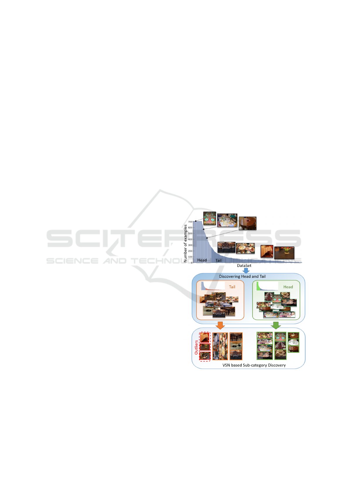
Figure 1: Distribution of class examples is a long tail dis-
tribution where class examples that happen more frequently
(e.g. table including plates) are located in the head and rare
examples (e.g. tables with chair) and outliers are in the tail.
Learning a monolithic model on this dataset may fail to de-
tect the tails. The goal is to improve learning accuracy by
discovering head and tail sub-categories.
Yancheshmeh, F., Chen, K. and Kämäräinen, J-K.
Hierarchical Deformable Part Models for Heads and Tails.
DOI: 10.5220/0006532700450055
In Proceedings of the 13th International Joint Conference on Computer Vision, Imaging and Computer Graphics Theory and Applications (VISIGRAPP 2018) - Volume 5: VISAPP, pages
45-55
ISBN: 978-989-758-290-5
Copyright © 2018 by SCITEPRESS – Science and Technology Publications, Lda. All rights reserved
45

Figure 1), but fail with the sub-categories having
sparse samples. Hence, modeling head and tail sub-
categories separately is necessary as suggested in ot-
her works (Gu et al., 2012; Dong et al., 2013; Zhu
et al., 2014). However, selecting right criteria to
group the objects properly remains an open problem.
Often long-tail examples spread among the clusters of
dominant ones and cannot form their own clusters or
outliers distort sub-category discovery.
In this work, we introduce a novel Hierarchi-
cal Deformable Part Model where we construct sub-
category hierarchy by alternating two sub-category
discovery approaches with complementary proper-
ties: bootstrapping and Visual Similarity Network
(VSN) (Shokrollahi Yancheshmeh et al., 2015). Boot-
strapping in the terms of DPM true positives and DPM
false negatives provides a rough division to the head
and tail parts. However, pair-wise similarity provides
better quality sub-categories for both dominant head
and ambiguous long-tail parts. The idea is to learn
strong models for the ones with enough examples and
share examples between rare models to improve de-
tection performance. For this intuitive approach the
hierarchy where all samples are used multiple times
establishes a strong data sharing principle (Salakhut-
dinov et al., 2011). Moreover, the hierarchy model na-
turally adapts to the number of examples - a small da-
taset allows only a shallow hierarchy while more ex-
amples allow deeper hierarchy and discovery of more
diverse sub-categories.
We make the following contributions:
• We propose a Hierarchical Deformable Part Mo-
del (HDPM) to capture long-tail distributions of
visual categories - our hierarchy is based on two
complementary and alternating approaches: i)
DPM bootstrapping and ii) Visual Similarity Net-
work based sub-category discovery.
• We adopt bootstrapping to make a coarse division
between the head and tail parts which are genera-
ted from true positives and false negatives of DPM
detection.
• We develop Visual Similarity Network (VSN)
based sub-category discovery to refine the sub-
categories of both head and tail parts.
• The baseline detector in our hierarchy is DPM.
We compare our method to other sub-category aware
works on the Pascal VOC 2007 benchmark where
our method outperforms other competitors. Moreo-
ver, we demonstrate the scalability of our method with
the ILSVRC 2014 Detection benchmark for which
our HDPM provides substantial performance boost as
compared to the conventional DPM. Our code will be
made publicly available.
2 RELATED WORK
Deformable Part Model (DPM) by Felzenswalb et
al. (Felzenszwalb et al., 2008; Felzenszwalb et al.,
2010) was a state-of-the-art approach in object de-
tection before the rise of convoluational neural net-
works (Girshick et al., 2014; Girshick, 2015; Ren
et al., 2015; Redmon et al., 2016). The seminal work
of Girshick et al. (Girshick et al., 2014) proposed the
Region-based Convolutional Neural Network model
(R-CNN) which has recently inspired many follow-
ups (Girshick, 2015; Ren et al., 2015; Redmon et al.,
2016). Interestingly, DPM achieves comparable accu-
racy to R-CNN if its HOG features are replaced by
activations of the CNN layers (Girshick et al., 2015;
Wan et al., 2015). CNN features require external trai-
ning data for optimization of the network parameters
(ILSVRC 2012 was used in (Girshick et al., 2015)).
In this work, our goal is to learn a model from the
scratch using only a moderate number of training ex-
amples and therefore we select the more conventional
HOG-based DPM (Felzenszwalb et al., 2010) as our
baseline detector. Experimental results of HDPM de-
monstrate the superiority of HDPM over recent met-
hods (Felzenszwalb et al., 2010; Malisiewicz et al.,
2011; Aghazadeh et al., 2012; Gu et al., 2012; Dong
et al., 2013; Zhu et al., 2014). Special cases of DPM
hierarchy have been introduced, for example, Ghiasi
and Fowlkes (Ghiasi and Fowlkes, 2014) used hierar-
chy of occlusion patterns to robust face detection, but
to the authors’ best knowledge our work is the first to
explicitly model intra-class diversities by introducing
hierarchical DPMs.
Long-Tail Distributions – Distributions of object
class examples in human captured images is not uni-
form, but certain classes and certain view points do-
minate datasets. For example, most of the people
stand in images, but they can also be assumed to have
a large number of unusual poses (e.g. a person riding
a horse). A practical solution is to balance a data-
set (Russakovsky et al., 2015). However it seems
difficult for collecting sufficient samples for tail sub-
categories. Reducing the sample size of dominant
sub-categories is more practical but it can have ne-
gative effect on detection performance. Performance
boost by modeling these rare sub-categories was rai-
sed by Salakhutdinov et al. (Salakhutdinov et al.,
2011) who introduced the data sharing principle: rare
classes borrow statistical strength from related classes
that have dense examples. The sharing was extended
to sub-categories that depict rare viewpoints by (Zhu
et al., 2014). In this work, we term both dominant
and rare appearance and viewpoints with a common
term of sub-category. While most of the works on
VISAPP 2018 - International Conference on Computer Vision Theory and Applications
46

long-tail visual detection use more traditional base-
line detection models, recently performance boost has
been reported also for the state-of-the-art CNN appro-
ach (Ouyang et al., 2016). In this work, we capture
sub-categories of the head and tail parts of long-tail
class distributions by adopting two principles: boots-
trapping and Visual Similarity Network (VSN) based
sub-category discovery.
Bootstrapping – Bootstrapping can be used to le-
arn different aspects of training data. For example,
mining hard negatives aims to distinguish two simi-
lar classes and mining hard positives works for co-
vering rarely encountered examples of a category. In
visual class detection bootstrapping is not new. Mi-
ning hard negatives (misclassified as positives) was
used already in the original HOG detector (Dalal and
Triggs, 2005) and later in DPM as well (Felzenszwalb
et al., 2008). In (Li et al., 2013) a term “relevant ne-
gatives” was introduced, but the principle is the same.
Our DPM learning also re-trains with hard negatives,
but we adopt bootstrapping to identify hard positives.
Zhu et al. (Zhu et al., 2014) construct candidate mo-
dels by training Exemplar-SVMs (Malisiewicz et al.,
2011) for each positive training example and selecting
a fixed amount of best scoring positive examples to
form a new sub-category training set. Greedy se-
arch is applied to select the best combination of the
DPMs, but the method is computationally expensive
due to a large number of the sub-models to be tested.
While their approach is bottom up, our bootstrapping
is top-down. We first construct a single DPM and se-
lect the false negatives to form a bootstrap set. Diffe-
rent from Zhu et al. (Zhu et al., 2014) bottom-up data
sharing, we propose a top-down hierarchy to discover
sub-categories by alternating visual similarity graph
based sub-category discovery and bootstrapping.
Sub-category Discovery – Sub-category discovery
and effective data exploitation are important for long-
tail distribution models in view of sparse samples in
long-tail sub-categories. Important research questions
arise: how to find sub-categories and how to effecti-
vely exploit small data in model learning? Sivic et
al. (an B.C. Russell et al., 2008) proposed a visual
Bag-of-Words based discovery of class hierarchy, but
their work assumed a number of dominant and balan-
ced categories. Sub-category (subordinate class) mi-
ning was proposed by Hillel and Weinshall (Hillel and
Weinshall, 2006) using generative models, but their
method cannot cope with viewpoint changes. In a
more recent work, Gu et al. (Gu et al., 2012) used a set
of seed images where other train images were aligned
using object boundaries and seed specific classifiers
were trained to represent sub-categories. The draw-
backs of their method are more demanding supervi-
sion in the terms of object boundary annotations and
unsupervised selection of good seeds. The method
by Aghazadeh et al. (Aghazadeh et al., 2012) avoided
strong supervision by using Exemplar-SVMs (Ma-
lisiewicz et al., 2011) to construct a classifier for
each example, but this exhaustive procedure limits
their method suitability only for moderate size data-
sets. (Aghazadeh et al., 2012) and (Malisiewicz et al.,
2011) did not particularly mine sub-categories, but
their methods relied on a large number of detectors
that together represent all aspects of the data. The
Exemplar-SVM based approach was extended by Zhu
et al. (Zhu et al., 2014) who also selected a number
of seed images for which Exemplar-SVM was em-
ployed, but they built stronger models by data sharing
where best scoring examples were added to the seed
sub-categories and DPMs trained as stronger detec-
tors. The DPMs were pruned by greedy search, but
the seed selection remains as a problem as well as
the non-adaptive addition of shared examples (a fixed
number). Dong et al. (Dong et al., 2013) proposed si-
milarity based sub-category mining, but their affinity
measure was based on Exemplar-SVN training with
again limits data set size to moderate. Alternatively,
Yu and Grauman (Yu and Grauman, 2014) postpo-
ned sub-category discovery to the testing phase and
used local neighborhood of each test sample. Pu et
al. (Pu et al., 2014) introduced intra-class grouping
(sub-categories) and data sharing penalties for Sup-
port Vector cost function to improve fine-grained ca-
tegorization.
Visual Similarity Networks – Hard decisions by
classifiers and clustering methods are always bia-
sed toward dominating patterns of data and there-
fore in this work we adopt a graph approach which
has recently gained momentum in vision applicati-
ons (Deng et al., 2014; Krause et al., 2015; John-
son et al., 2015; Rematas et al., 2015; Rubinstein
et al., 2016). A graph represents multiple latent and
even subtle connections between samples without the
need of hard decisions. We adopt a special structure
denoted as Visual Similarity Network (VSN) where
the links between vertices denote the strength of a
pair-wise similarity between two images. One of the
first VSN models was the matching graph structure
by Philbin and Zisserman (Philbin and Zisserman,
2008), but it was developed for specific object ma-
tching as link between local features connected two
different viewpoints of the same object. In parallel,
Kim et al. (Kim et al., 2008) seeded the term Vi-
sual Similarity Network and proposed a method to
construct a graph representing visual categories. Re-
cently, more advanced Visual Similarity Network ap-
proaches were proposed in (Isola et al., 2015; Shok-
Hierarchical Deformable Part Models for Heads and Tails
47

Figure 2: The HDPM workflow: bootstrapping and VSN sub-category discovery alternate along the hierarchy levels (the steps
2 and 3 repeat). The best combination of DPM models are selected in section 3.3.
rollahi Yancheshmeh et al., 2015; Zhou et al., 2015).
Isola et al. (Isola et al., 2015) VSN represents ca-
tegory transformations, e.g. from a raw tomato to
a rotten tomato while Shokrollahi et al. (Shokrol-
lahi Yancheshmeh et al., 2015) and Zhou et al. (Zhou
et al., 2015) provided pair-wise similarity in a full
connected manner. They both constructed a network
from local features that align over geometric transfor-
mations and therefore capture viewpoint changes. In
this work, we adopt the VSN approach in (Shokrol-
lahi Yancheshmeh et al., 2015) and adapt it for sub-
category discovery by accumulating local features to
represent category specific landmarks.
3 HIERARCHICAL DPM
Our Hierarchical DPM (Figure 2) constructs hierar-
chy where at the top we have a root model learned
using all training examples (Step 1). Branches re-
present division of images to sub-categories by two
alternating procedures: 1) Step 2 – bootstrapping
(Section 3.1) and 2) Step 3 – Visual Similarity Net-
work (VSN) sub-category discovery (Section 3.2). As
we move from a root to leaves, the sub-categories re-
present more exclusive distinctions. Intuitively boot-
strapping will provide a coarse division to long-tail
distribution’s head and tail parts. VSN sub-category
discovery refines both parts by identifying less domi-
nant sub-categories that would otherwise be suppres-
sed by dominating ones.
The input of HDPM is a set of N training examples
S =
{
I, b, c
}
n=1,...,N
where I
n
denotes the nth training
image, b
n
bounding box coordinates of a class with
the label c. Each class contains N
c
training samples
and HDPM
c
:s are constructed independently. The ba-
seline model used in each tree node is Deformable
Part Model (DPM) (Felzenszwalb et al., 2008; Fel-
zenszwalb et al., 2010)
M
c
DPM
= DPM (S
c
, S
neg
) (1)
where S
c
∈ S is a set of positive examples for the class
c and S
neg
is a set of negative examples (images of all
other classes S
neg
= S \ S
c
in our experiments).
3.1 Bootstrapping
A known characteristic of the Latent SVM (Felzen-
szwalb et al., 2008) algorithm in DPM is that it can
effectively learn a dominating sub-category from S
c
,
but cannot represent less dominating sub-categories
and suffers from more than one competing domi-
nant sub-category. To cope with multiple domina-
ting sub-categories, DPM clusters box aspect ratios
of the input bounding boxes to M clusters for which
separate DPMs are trained referring to components in
the DPM terminology. Our hierarchy replaces heu-
ristic discovery of components by data-driven sub-
categorization.
The baseline model in (1) is trained for remaining
training examples after each branch in the tree. Then,
we test the trained model M
c
on the positive exam-
ples to divide them into two bootstrap sets: domi-
nant sub-category examples (true positives) S
+
c
and
rare sub-category examples (false negatives) S
−
c
. In
the next step, the both sets are refined to the next le-
vel sub-categories by Visual Similarity Network sub-
category discovery (Section 3.2). In addition to VSN
we also train two bootstrapped DPMs using the two
sets:
M
c
+
DPM
= DPM

S
+
c
, S
neg

M
c
−
DPM
= DPM

S
−
c
, S
neg

.
(2)
VISAPP 2018 - International Conference on Computer Vision Theory and Applications
48

In our preliminary experiments we evaluated two va-
riants by adding not detected or detected examples
to the negative set respectively, S
+
neg
= S
neg
∪ S
−
c
and
S
−
neg
= S
neg
∪ S
+
c
, but found this inferior to using only
S
neg
.
3.2 Visual Similarity Network for
Sub-Categories
The motivation behind VSN based sub-category dis-
covery is to identify both appearance sub-categories,
e.g. enduro and scooter motorbikes, and viewpoint
sub-categories, e.g. frontal and side views of cars.
If the number of samples is small for these sub-
categories (long-tail sub-categories), we need to adopt
an approach that retains all pair-wise image similari-
ties. A suitable data structure is the similarity graph
which has been used in similar tasks in the recent
works (Isola et al., 2015; Shokrollahi Yancheshmeh
et al., 2015; Zhou et al., 2015). We adopt Visual Si-
milarity Network (VSN) by Shokrollahi et al. (Shok-
rollahi Yancheshmeh et al., 2015) and adapt it for our
problem by introducing class specific landmark accu-
mulation.
The main component of (Shokrollahi Yan-
cheshmeh et al., 2015) is a cost function
C(I
a
, I
b
) = λ
1
C
match
(I
a
, I
b
) + λ
2
C
dist.
(I
a
, I
b
) , (3)
which computes the matching cost of two images, I
a
and I
b
, using feature correspondence with matching
cost C
match
and spatial distortion cost C
dist
. The ma-
tching cost denotes similarity in a feature space (e.g.
SIFT) and distortion cost how well the features can
be aligned in the spatial domain. Minimization of the
cost function (3) is cast as a generalized assignment
problem:
maximize
∑
i
∑
j
s
i j
a
i j
subject to
∑
j
a
i j
≤ 1 i = 1, . . . , N
a
∑
i
a
i j
≤ 1 j = 1, . . . , N
b
a
i j
∈
{
0, 1
}
, (4)
where a
i j
are binary assignments between the features
i = 1, . . . , N
a
of the image I
a
and j = 1, . . . , N
b
of I
b
.
The assignment constraints require at most one match
between each feature and s
i j
:s are similarity values in
[0, 1] that combine the previously defined feature and
distortion costs into a single value
S(i, j) = e
C(i, j)
= e
λ
1
D
F
(i, j)
e
λ
2
D
X
(i, j)
= S
F
(i, j)S
X
(i, j) .
(5)
D
X
is the distance in the spatial space and D
F
denotes
the distance in the feature space. For solving the opti-
mization problem Shokrollahi et al. (Shokrollahi Yan-
cheshmeh et al., 2015) proposed to replace the cost
values with rank-order statistics yielding to fast ap-
proximation sketched in Algorithm 1 where the trans-
formation T is parameterized with a translation vector
(t
x
,t
y
), rotation θ and uniform scaling s.
Algorithm 1: Generalized assignment approx. solution.
1: Compute the feature distance matrix D
F
N
a
×N
b
(e.g.,
dense SIFT).
2: On each row of D
F
set the K smallest to 1 and 0 other-
wise.
3: S
X
= 0.
4: for i = 1 : N
a
(features of I
a
) do
5: Compute the distance from x
(a)
i
to T (x
(b)
j
) for j =
1, . . . , K non-zero entries of D
F
and if D
X
(i, j) ≤ τ
X
then set S
X
(i, j) = 1 and break.
6: end for
7: return the number of non-zero terms in S
X
3.2.1 Object Landmark Driven Similarity
The main problem of Algorithm 1 is that in the pre-
sence of background clutter it can get stuck to ma-
tching backgrounds (background-to-background ma-
tching) or object-to-background matching instead of
the desired object-to-object matching. Our solution is
two-fold: i) we mask features outside object region
by bounding boxes and ii) accumulate features that
match in multiple images to produce a refined set of
class specific landmarks.
We adopt otherwise the parameter settings from
the original work, but run an accumulation procedure
in Algorithm 2. The algorithm retains only the lo-
Algorithm 2: Accumulation of I
a
landmark scores.
1: S
X
acc
= 0.
2: for n = 1 : N
c
in S
c
do
3: Compute Nelder-Mead optimization (max search) of
the transformation matrix T parameters using Algo-
rithm 1 as the target function.
4: S
X
acc
= S
X
acc
+ S
X
5: end for
6: return Remove other than the B best features of I
a
cal features that are verified by multiple training set
images and therefore removes object-to-background
and background-to-background matches effectively.
Using the verified set of local features, object specific
landmarks, we can re-execute Algorithm 1 and com-
pute the affinity matrix representing pair-wise mat-
ches between all images using the verified landmarks:
Hierarchical Deformable Part Models for Heads and Tails
49

A
c
a f f
=




kS
X
I
1
,I
1
k kS
X
I
1
,I
2
k kS
X
I
1
,I
3
k . . . kS
X
I
1
,I
N
c
k
.
.
.
.
.
.
.
.
. . . .
.
.
.
kS
X
I
N
c
,I
1
k kS
X
I
n
c
,I
2
k kS
X
I
2
,I
3
k . . . kS
X
I
N
c
,I
N
c
k




(6)
where k · k is the number of non-zero terms in S
X
and now represents similarity in [0, B]. For our expe-
riments we set B = 80, but this selection does not have
drastic effect to the performance as long as B ≥ 20.
3.2.2 Spectral Sub-categories
The next step is to discover sub-categories in the
full connected graph defined by the affinity ma-
trix A
c
a f f
in (6). For this task we adopt the self-
tuning spectral clustering by Zelnik-Manor and Pe-
rona (Zelnik-Manor and Perona, 2004) which ex-
tends the original spectral clustering of Ng et al. (Ng
et al., 2001) by adding unsupervised selection for the
spectral scale and number of clusters.
Similarity values in (6) represent pair-wise simi-
larity as an integer where B denotes high similarity
(all landmarks match) and 0 low similarity (no mat-
ches). Self-tuning spectral clustering is based on pre-
computed node distance matrix and therefore we con-
vert integer similarities to rank-order distances (the
super- and the sub-scripts of the affinity matrix omit-
ted for clarity):
D
i j
=
N
c
rank(A
i j
, sort(A
i,:
))
. (7)
where N
c
is the highest rank (distance is 1) and 1 is
the lowest (distance N
c
).
The scaled affinity matrix is computed from the
rank-order distance matrix
ˆ
A
i j
= exp
−D
2
i j
σ
i
σ
j
!
(8)
where
σ
i
= D
iK
(9)
where D
iK
is “distance” to the K:th neighbor of i:th
entry (K = 10 in our experiments). Moreover,
ˆ
A
ii
= 0.
For the normalized affinity matrix the C largest eigen
vectors are selected and the rotation R that aligns the
matrix formed from the eigen vectors to the canonical
coordinate system and the number of clusters is iden-
tified by selecting the number of clusters that provides
the minimal alignment cost. The number of clusters
from 2 to 15 were tested in our experiments. See Fi-
gure 3 for illustrations of the found sub-categories.
Figure 3: VSN sub-category discovery for the head and tail
parts of the VOC2007 bicycle class and ILSVRC2014 ca-
mel. Note how the head sub-categories are more evident and
tail sub-categories represent rare examples (upside-down
bicycle, resting camel). Outliers not detected by our system
are marked red and often represent ambiguous annotation
(e.g. only a bicycle handle, heavily occluded camel, extre-
mely poor resolution).
Similar to the bootstrapping in Section 3.1 we
train separate DPMs for each VSN sub-category c(1),
c(2), . . . , c(C)
M
c
DPM
c(i)
= DPM

S
c(i)
, S
neg

. (10)
Since the bootstrapping and VSN sub-category disco-
very steps alternate (Figure 2) the sub-category DPMs
give raise to new division to head and tail sets by boot-
strapping and the process continues similarly until too
few examples to train DPMs (e.g. ≤ 15 images for
each sub-category). In our experiments, we fixed the
maximum level to 8.
3.3 Model-Selection
In validation time, we select the best set of DPM mo-
dels in (Figure 2). This procedure can be very time
consuming since all possible combination for n num-
ber of DPM models is
∑
n
r=1
n!
r!(n−r)!
and thus not com-
putationally effective. Instead, we take advantage of
the hierarchical tree where we expect to have the mo-
dels of dominant subcategories on the right branch
(green in Figure 2) and long tails’ on the left branch
(orange in Figure 2). Therefore, we should have the
strongest models on the right side and if the left side
learned something new, then it will be added. Thus,
we first explore the best models combination from the
right side that gives the maximum score on validation
set, next we give the selected set to the left side and
repeat the process again. The output will be our final
selected set of models.
VISAPP 2018 - International Conference on Computer Vision Theory and Applications
50

Table 1: Pascal VOC 2007 comparison (AP in %) of state-of-the-art sub-category aware methods.
∗
DP-DPM Uses external
training data (1.2M image ILSVRC 2012 training set).
Method aero bike bird boat bott bus car cat chair cow tabl dog horse mbike pers plant sheep sofa train tv mAP
DPM (Felzenszwalb et al., 2010) 28.7 55.1 6.0 14.5 26.5 39.7 50.2 16.3 16.5 16.6 24.5 5.0 45.2 38.7 36.2 9.0 17.4 22.8 34.1 38.4 27.1
DPMv5 Website 32.1 60.2 10.5 14.0 30.0 54.0 57.0 24.7 22.6 26.8 29.1 8.6 59.8 46.7 41.4 13.4 22.1 34.4 44.3 44.5 33.8
DPMv5-reproduced 32.8 59.3 10.9 14.1 29.2 52.6 57.8 27.5 23.1 24.6 30.8 13.0 61.6 46.6 40.2 13.0 19.1 31.2 46.3 44.4 33.9
ESVM (Malisiewicz et al., 2011) 20.8 48.0 7.7 14.3 13.1 39.7 41.1 5.2 11.6 18.6 11.1 3.1 44.7 39.4 16.9 11.2 22.6 17.0 36.9 30.0 22.7
MCIL (Aghazadeh et al., 2012) 33.3 53.6 9.6 15.6 22.9 48.4 51.5 16.3 16.3 20.0 23.8 11.0 55.3 43.8 36.9 10.7 22.7 23.5 38.6 41.0 29.8
MCM (Gu et al., 2012) 33.4 37.0 15.0 15.0 22.6 43.1 49.3 32.8 11.5 35.8 17.8 16.3 43.6 38.2 29.8 11.6 33.3 23.5 30.2 39.6 29.0
DPM-AGS (Dong et al., 2013) 34.7 61.4 11.5 18.6 30.0 53.8 58.8 24.7 24.7 26.8 31.4 13.8 61.4 49.2 42.2 12.9 23.9 38.5 50.8 45.5 35.7
DPM-LTS (Zhu et al., 2014) 34.1 61.2 10.1 18.0 28.9 58.3 58.9 27.4 21.0 32.3 34.6 15.7 54.1 47.2 41.2 18.1 27.2 34.6 49.3 42.2 35.7
HDPM (ours) 35.8 61.6 11.9 17.2 30.5 53.9 59.1 29.2 23.8 27.5 37.0 15.3 62.4 48.4 42.4 16.3 21.2 35.1 47.7 45.8 36.1
DP-DPM (Girshick et al., 2015)
∗
44.6 65.3 32.7 24.7 35.1 54.3 56.5 40.4 26.3 49.4 43.2 41.0 61.0 55.7 53.7 25.5 47.0 39.8 47.9 59.2 45.2
4 EXPERIMENTS
4.1 Datasets and Settings
To make our method comparable with the similar
works (Zhou et al., 2015; Dong et al., 2013), we eva-
luated HDPM on the PASCAL VOC 2007 dataset.
Pascal VOC 2007 contains 20 categories with 9, 963
images in total. The dataset is divided into ‘train-
val’ and ‘test’ subsets including 5011 and 4952 ima-
ges, respectively. In our experiments, we follow the
protocol in (Zhou et al., 2015) and report the results
for the ‘test’ subset. In the experiments on the VOC
2007 benchmark, we set the number of components in
DPM detector to 2 and we continue constructing the
HDPM hierarchy up to the level 8.
We also evaluate the performance of the propo-
sed method on the ILSVRC2014 detection task to
test scalability. ILSVRC 2014 detection set contains
456, 567 training images, 20, 121 validation images,
and 40, 152 test images. There are 200 categories
and the number of positive training images per cate-
gory varies between 461 and 67, 513. The number
of negative training images per category is between
42, 945 and 70, 626. The ground truth are released
only for the training and validation data and for test
data we submitted our results to the evaluation ser-
ver (one submission was made for each class). To
speed up the computation with ILSVRC we made the
following compromises: a) the maximum number of
negative examples was set to the number of positive
images per each class, b) the number of DPM com-
ponents was fixed to 1 and c) HDPM hierarchy was
computed only up to the level L3. These compromi-
ses allowed computation of 200 HDPMs within one
week.
With the both datasets, we first constructed
HDPMs for each class using the training exam-
ples, and then selected the best combination of the
sub-category DPMs using the validation examples
(Section 3.3). For constructing the VSNs, we first
cropped images inside the bounding boxes and sca-
led them to the size of 200 × 200 pixels keeping as-
pect ratios. Secondly, we executed spectral cluste-
ring (Zelnik-Manor and Perona, 2004) that automa-
tically selected the number of clusters and provided
sub-category assignments for each image. In all ex-
periments, we set the search range for the number
of clusters to 2 − 15, and the method typically pro-
vided 2−4 on each hierarchy level. We employed the
standard Non-Maximum Suppression (NMS) on the
detected candidates of bounding boxes. The evalu-
ation metric was Average Precision (AP) and mean
of Average Precision (mAP) without contextual re-
scoring.
4.2 Comparison with State-of-the-Arts
In this experiment, we compared our method to ot-
her published sub-category aware methods on the
Pascal VOC 2007 dataset and using only the pro-
vided training and validation set images in model
training: Exemplar-SVM (ESVM) by Malisiewicz et
al. (Malisiewicz et al., 2011), Multi-Component Mo-
del (MCM) by Gu et al. (Gu et al., 2012), Mixture
Component Identification and Learning (MCIL) by
Aghazadeh et al. (Aghazadeh et al., 2012) Ambiguity
Guided Graph Shift DPM (DPM-AGS) by Dong et
al. (Dong et al., 2013) and Long-Tail Subcategories
DPM (DPM-LTS) by Zhu et al. (Zhu et al., 2014).
The results are shown in Table 1. Since our baseline
model is based on the DPM version 5 (DPMv5), we
also report results achieved in our own experiments
as well as the results reported in (Felzenszwalb et al.,
2010). The results slightly vary due to parallel execu-
tion since computing the cost function gradient varies
with different numbers of threads. In addition, we re-
port the results for the the deep DPM where the HOG
features are replaced with activations of the full Ima-
geNet dataset trained neural network AlexNet (DP-
DPM) by Girshick et al. (Girshick et al., 2015).
Our model achieved the best average precision
(AP) for 8 out of the 20 categories and the best overall
mean average precision (mAP). By comparing our re-
Hierarchical Deformable Part Models for Heads and Tails
51

Figure 4: Per class boost in ILSVRC2014 detection task using HDPM over DPM (blue: > 1, green: ≈ 1, orange: < 1).
sults to the two similar and recent works, DPM-AGS
and DPM-LTS, it is evident that the upper limit of
performance using HOG features and only the provi-
ded data is almost reached. There is a clear difference
as compared to DP-DPM, but their method uses the
additional massive ImageNet dataset for training the
CNN feature extraction network.
4.3 Large Scale Scalability on the
ImageNet 200
Figure 4 shows the proportional improvement using
HDPM over DPM for the 200 ILSVRC2014 detection
task classes. It is noteworthy, that using our restricted
settings we improved performance for 143 out of 200
categories. For 30 classes the boost was > 2× and
only for 12 classes the performance degraded below
0.5. The mAP values were 9.84% for HDPM and
8.54% for DPM providing average improvement of
15% and median improvement of 40% being clearly
significant. The results are on pair with the state-of-
the-art before the era of CNNs. Per class accuracies
are available in appendix.
5 CONCLUSIONS
We proposed HDPM to address the problem of long-
tail distributions of visual class examples. Our mo-
del achieved superior accuracy to other proposed sub-
category aware DPM-based models and provides sca-
lability to large scale problems. In our future work,
we will replace the standard HOG DPM with the more
recent Deep DPM (Girshick et al., 2015) to bene-
fit from the performance of data optimized features
and we will investigate computationally more power-
ful bootstrapping and SVN construction.
REFERENCES
Aghazadeh, O., Azizpour, H., Sullivan, J., and Carlsson, S.
(2012). Mixture component identification and lear-
ning for visual recognition. In ECCV.
an B.C. Russell, J. S., Zisserman, A., Freeman, W., and
Efros, A. (2008). Unsupervised discovery of visual
object class hierarchies. In CVPR.
Dalal, N. and Triggs, B. (2005). Histograms of oriented
gradients for human detection. In CVPR.
Deng, J., Ding, N., Jia, Y., Frome, A., Murphy, K., Bengio,
S., Li, Y., Neven, H., and Adam, H. (2014). Large-
scale object classification using label relation graphs.
In ECCV.
Dong, J., Xia, W., Chen, Q., Feng, J., Huang, Z., and Yan,
S. (2013). Subcategory-aware object classification. In
CVPR.
Felzenszwalb, P., Girshick, R., McAllester, D., and Rama-
nan, D. (2010). Object detection with discriminatively
trained part-based models. IEEE PAMI, 32(9):1627–
1645.
Felzenszwalb, P., McAllester, D., and Ramanan, D. (2008).
A discriminatively trained, multiscale, deformable
part model. In CVPR.
Ghiasi, G. and Fowlkes, C. (2014). Occlusion coherence:
Localizing occluded faces with a hierarchical defor-
mable part model. In CVPR.
Girshick, R. (2015). Fast R-CNN. In ICCV.
Girshick, R., Donahue, J., Darrell, T., and Malik, J. (2014).
Rich feature hierarchies for accurate object detection
and semantic segmentation. In CVPR.
Girshick, R., Iandola, F., Darrell, T., and Malik, J. (2015).
Deformable part models are convolutional neural net-
works. In CVPR.
VISAPP 2018 - International Conference on Computer Vision Theory and Applications
52

Gu, C., Arbelaez, P., Lin, Y., Yu, K., and Malik, J. (2012).
Multi-component models for object detection. In
ECCV.
Hillel, A. and Weinshall, D. (2006). Subordinate class re-
cognition using relational object models. In NIPS.
Isola, P., Lim, J., and Adelson, E. (2015). Discovering states
and transformations in image collections. In CVPR.
Johnson, J., Krishna, R., Stark, M., Li, L.-J., Shamma, D.,
Bernstein, M., and Fei-Fei, L. (2015). Image retrieval
using scene graphs. In CVPR.
Kim, G., Faloutsos, C., and Hebert, M. (2008). Unsupervi-
sed modeling of object categories using link analysis
techniques. In CVPR.
Krause, J., Jin, H., Yang, J., and Fei-Fei, L. (2015).
Fine-grained recognition without part annotations. In
CVPR.
Li, X., Snoek, G., Worring, M., D.Koelma, and Smeulders,
A. (2013). Bootstrapping visual categorization with
relevant negatives. IEEE Trans. on Multimedia, 15(4).
Malisiewicz, T., Gupta, A., and Efros, A. (2011). Ensemble
of exemplar-SVMs for object detection and beyond.
In ICCV.
Ng, A., Jordan, M., and Weiss, Y. (2001). On spectral clus-
tering: Analysis and an algorithm. In NIPS.
Ouyang, W., Wang, X., Zhang, C., and Yang, X. (2016).
Factors in finetuning deep model for object detection
with long-tail distribution. In CVPR.
Philbin, J. and Zisserman, A. (2008). Object mining using
a matching graph on very large image collections. In
Indian Conference on Computer Vision, Graphics and
Image Processing.
Pu, J., Jiang, Y.-G., Wang, J., and Xue, X. (2014). Which
looks like which: Exploring inter-class relationships
in fine-grained visual categorization. In ECCV.
Redmon, J., Divvala, S., Girshick, R., and Farhadi, A.
(2016). You only look once: Unified, real-time ob-
ject detection. In CVPR.
Rematas, K., Fernando, B., Dellaert, F., and Tuytelaars, T.
(2015). Dataset fingerprints: Exploring image col-
lections through data mining. In CVPR.
Ren, S., He, K., Girshick, R., and Sun, J. (2015). Faster R-
CNN: Towards real-time object detection with region
proposal networks. In NIPS.
Rubinstein, M., Liu, C., and Freeman, W. (2016). Joint in-
ference in weakly-annotated image datasets via dense
correspondence. Int J Comp Vis, 119:23–45.
Russakovsky, O., Deng, J., Su, H., Krause, J., Satheesh, S.,
Ma, S., Huang, Z., Karpathy, A., Khosla, A., Bern-
stein, M., Berg, A. C., and Fei-Fei, L. (2015). Image-
Net Large Scale Visual Recognition Challenge. Int J
Comp Vis, 115(3):211–252.
Salakhutdinov, R., Torralba, A., and Tenenbaum, J. (2011).
Learning to share visual appearance for multiclass ob-
ject detection. In CVPR.
Shokrollahi Yancheshmeh, F., Chen, K., and K
¨
am
¨
ar
¨
ainen,
J.-K. (2015). Unsupervised visual alignment with si-
milarity graphs. In CVPR.
Wan, L., Eigen, D., and Fergus, R. (2015). End-to-end inte-
gration of a convolutional network, deformable parts
model and non-maximum suppression. In CVPR.
Yu, A. and Grauman, K. (2014). Predicting useful neig-
hborhoods for lazy local learning. In NIPS.
Zelnik-Manor, L. and Perona, P. (2004). Self-tuning
spectral clustering. In NIPS.
Zhou, T., Lee, Y., Yu, S., and Efros, A. (2015). Flow-
Web: Joint image set alignment by weaving consis-
tent, pixel-wise correspondences. In CVPR.
Zhu, X., Anguelov, D., and Ramanan, D. (2014). Captu-
ring long-tail distributions of object subcategories. In
CVPR.
Hierarchical Deformable Part Models for Heads and Tails
53

APPENDIX
Figure 5: AP over the first 200 categories (synsets) of ImageNet test set (part1).
VISAPP 2018 - International Conference on Computer Vision Theory and Applications
54

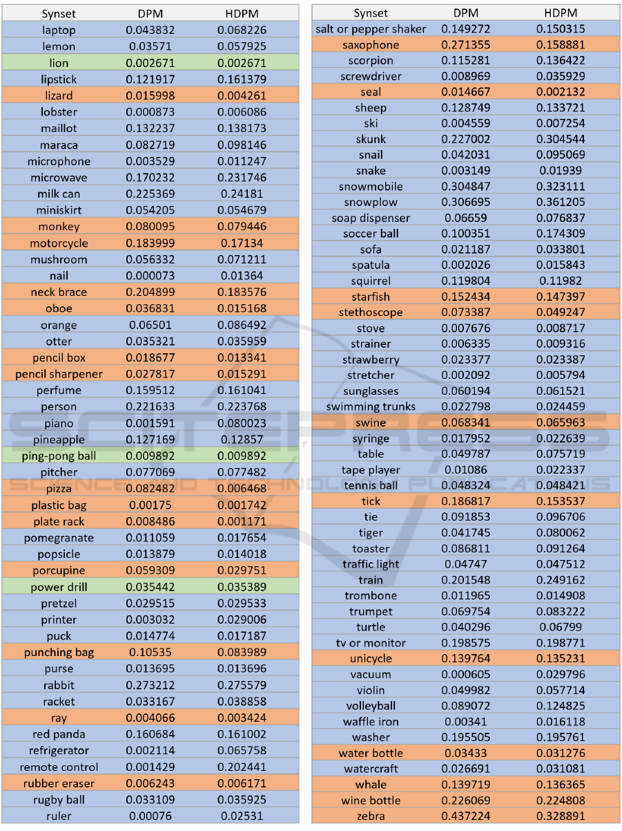
Figure 6: AP over next 200 categories of ImageNet test set (part2).
Hierarchical Deformable Part Models for Heads and Tails
55