
Brain Tumor Segmentation in Magnetic Resonance Images using Genetic
Algorithm Clustering and AdaBoost Classifier
Gustavo C. Oliveira
1
, Renato Varoto
2
and Alberto Cliquet Jr.
1,2,3
1
University of São Paulo Interunits Graduate Program in Bioengineering, University of São Paulo, São Carlos - SP, Brazil
2
Department of Orthopedics and Traumatology, University of Campinas (UNICAMP), Campinas - SP, Brazil
3
Department of Electrical and Computer Engineering, University of São Paulo, São Carlos - SP, Brazil
Keywords:
Image Segmentation, Glioma, Genetic Algorithm, AdaBoost Classifier.
Abstract:
We present a technique for automatic brain tumor segmentation in magnetic resonance images, combining
a modified version of a Genetic Algorithm Clustering method with an AdaBoost Classifier. In a group of
42 FLAIR images, segmentations produced by the algorithm were compared to the ground truth information
produced by radiologists. The mean Dice similarity coefficient reached by the algorithm was 70.3%. In
most cases, the AdaBoost classifier increased the quality of the segmentation, improving, on average, the
DSC in about 10%. Our implementation of the Genetic Algorithm Clustering method presents improvements
compared to the original method. The use of a fixed, small number of groups and smaller population allowed
for less computational effort. In addition, adaptive restriction in the initial segmentation was achieved by using
the information of the groups with highest and 2nd-highest mean intensities. By exploring intensity and spatial
information of the pixels, the AdaBoost classifier improved segmentation results.
1 INTRODUCTION
Glioma is a type of brain tumor that originates in
the glial cells, which support and surround neurons
in the brain. Growing within the tissue of the brain
and often mixing with healthy areas, it’s the most
frequent primary brain tumor in adults, representing
33% of all cases. By pressing on the spinal cord or
the brain, gliomas can cause many symptoms, such
as seizures, personality changes, weakness in the face
or limbs, problems with speech, vision loss and dizzi-
ness. In its less aggressive form, known as low-grade
gliomas, patients have a life expectancy of several
years, and in its more aggressive form, known as high-
grade gliomas, patients have a median survival rate of
two years or less. The most common treatment for
gliomas is surgery, which may be followed by radia-
tion therapy and chemotherapy (Menze et al., 2015;
Johns Hopkins Medicine Health Library, 2017).
Diagnosis of glioma tumors involves an analysis
of the patient’s medical history, neurological exams
and scans of the brain – magnetic resonance imaging
and computed tomography. Throughout the treatment
process, imaging protocols are used to follow disease
progression and evaluate the success of the chosen
strategy. Analysis of those images usually relies on
rudimentary quantitative measures or qualitative cri-
teria – such as the largest diameter visible from ax-
ial images of the lesion or presence of characteristic
hyper-intense tissue (Menze et al., 2015; Johns Hop-
kins Medicine Health Library, 2017).
In this context, the development of computer
aided-diagnosis (CAD) systems that can automati-
cally analyze brain tumor scans and replace the cur-
rent evaluation methods with more reproducible and
accurate measurements could significantly improve
the diagnosis, treatment and follow-up processes by
providing standardized criteria for tumor characteri-
zation and time efficiency (Menze et al., 2015; Em-
blem et al., 2009). More specifically, CADs could
perform the segmentation task, separating the differ-
ent tumor tissues from healthy brain tissue, to extract
the patient specific clinical information, along with
their diagnostic features. In the last years, a great vari-
ety of segmentation methods was proposed, combin-
ing threshold-based, model-based, region-based and
pixel classification techniques (Gordillo et al., 2013).
Comparing these methods, however, is problematic,
since they are usually validated with different perfor-
mance metrics, on small and private datasets and us-
ing different imaging modalities (Menze et al., 2015).
To overcome these difficulties, the Multimodal
Oliveira, G., Varoto, R. and Jr., A.
Brain Tumor Segmentation in Magnetic Resonance Images using Genetic Algorithm Clustering and AdaBoost Classifier.
DOI: 10.5220/0006534900770082
In Proceedings of the 11th International Joint Conference on Biomedical Engineering Systems and Technologies (BIOSTEC 2018) - Volume 2: BIOIMAGING, pages 77-82
ISBN: 978-989-758-278-3
Copyright © 2018 by SCITEPRESS – Science and Technology Publications, Lda. All rights reserved
77
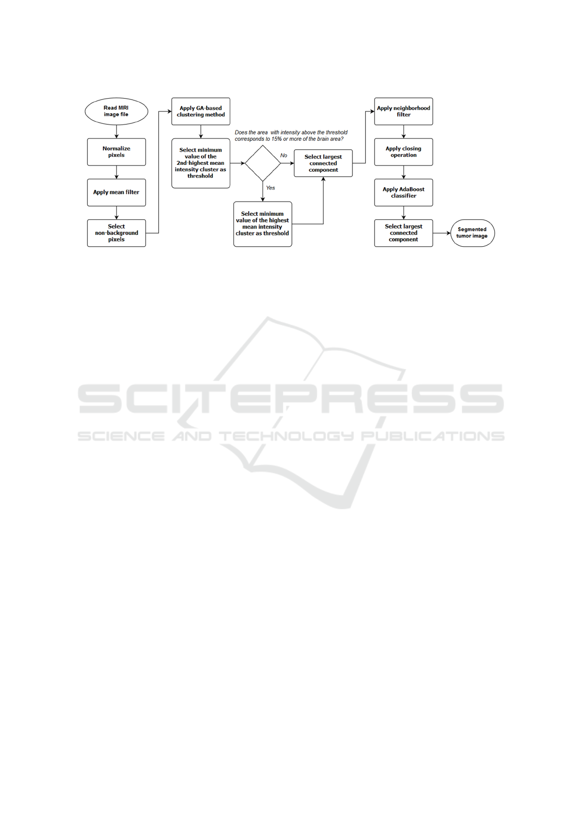
Figure 1: Flowchart of the algorithm.
Brain Tumor Image Segmentation (BRATS) chal-
lenge was organized. In this challenge, 20 state-of-
art algorithms were applied to the same dataset and
evaluated in three different tasks: segmentation of
the “whole” tumor (including edema, non-enhancing
solid core, active core and non-solid core), segmen-
tation of the tumor “core” (including all classes ex-
cept edema), and segmentation of the “active tumor”
(containing only the “active core”). It was found that
no single method ranked in the top five for all tasks -
different algorithms performed best for different sub-
regions. The development of algorithms for brain tu-
mor segmentation continues to attract interest of the
research community (Menze et al., 2015).
Kole and Halder proposed an automatic method
for brain tumor detection and isolation of tumor cells
from magnetic resonance images (MRI) using a ge-
netic algorithm-based clustering method (Kole and
Halder, 2012). In this paper, an extension of their
technique is presented, combining their clustering
method with morphological operation, filters and an
AdaBoost classifier.
2 MATERIALS AND METHODS
2.1 Algorithm
The flowchart presented in Figure 1 gives an overview
of the proposed technique, which operates as fol-
lows. First, pixels in the image are normalized and
a 3x3x3 mean filter is applied. Non-background pix-
els are then selected and grouped into clusters ac-
cording to their intensity values using the genetic
algorithm (GA)-based clustering method (Kole and
Halder, 2012).
Let K represent the number of clusters that the
pixels of the image will be divided into. K ranges
from 2 to 5 - i.e. pixels will be divided into 2, 3, 4 and
5 clusters. In the GA-based clustering method, each
chromosome of the population consists of K numbers,
intensity values which represent the centers of each
cluster. At each generation, a fitness function is com-
puted in order to find and select the center values that
best divide the pixels into K clusters by minimizing
intra-cluster spread. The next generation is then cre-
ated using mutation and cross-over processes. This
is repeated through several iterations. Then K is in-
creased, new chromosomes are generated and the evo-
lutionary process is repeated. This continues until K
reaches its final value. Finally, pixels are grouped us-
ing the most appropriate number of clusters, which is
the one that minimizes the validity index (Kole and
Halder, 2012). Overall, the method can be summa-
rized in the following steps:
1. For each number of groups K, repeat steps 2 to 7.
2. Generate initial values of each chromosome of the
population.
3. Calculate the fitness value of each chromosome.
4. Preserve the chromosome with highest fitness
value found so far.
5. Select chromosomes using the Roulette Wheel al-
gorithm.
6. Create chromosomes of the next generation
through mutation and cross-over.
7. Until termination condition is reached, repeat
steps 3 to 6.
8. Compute the clustering validity index for the
fittest chromosome of all values of K.
9. Cluster pixels using the value of K that minimizes
the validity index.
For more details, please refer to the original article
(Kole and Halder, 2012).
BIOIMAGING 2018 - 5th International Conference on Bioimaging
78

After finding the clusters, thresholding is per-
formed to obtain a binary image. Selection of the
threshold value is based on the clusters: the first
choice is to use the minimum value of the cluster
with 2nd highest mean intensity. Pixels with inten-
sity value above the threshold are marked as tumor
(i.e. they’re assigned the value “1”), whereas pixels
with intensity value below the threshold are marked
as background (i.e. they’re assigned the value “0”). If
the thresholding operation results in a segmentation
that selects more than 15% of the area of the brain as
tumor, then the first binary image is abandoned and
the minimum value of the cluster with highest mean
intensity is chosen as the threshold value. The thresh-
old operation is repeated, producing a new binary im-
age.
Once the binary image is produced, the program
selects the largest connected component and applies
to it a neighborhood filter. This filter computes, for
each pixel, the number of tumor pixels that are 8-
connected to it, i.e. the number of tumor pixels that
touches one of the edges or corners of the pixel. If
this number is 4 or more, then the current pixel is in-
cluded. If it’s 2 or less, the current pixel is excluded
or not included in the tumor area (Gibbs et al., 1996;
Sonka et al., 2014). Following the filtering step, holes
in the segmented area are removed by applying the
morphological closing operation iteratively, using a
small disk as the structuring element.
Finally, an AdaBoost classifier is used to improve
the segmentation. The AdaBoost algorithm is a tech-
nique used to create a strong, accurate classifier by
combining weak classifiers, assumed to be better than
random guessing in correctly classifying the data. For
a training set of multidimensional data points, a clas-
sifier will assign to each data point a label, either +1
or -1. An exponential error function is used to rank
all the weak classifiers based on the number of cor-
rect and incorrect classifications. AdaBoost proceeds
by systematically extracting one classifier of the pool
in each of the iterations, by focusing on the ones that
can help with the misclassified data points. After ex-
tracting a weak classifier, AdaBoost assigns a weight
to it. The stronger classifier is then given by the group
of extracted weak classifiers combined with their as-
signed weights (Freund and Schapire, 1995; Schapire,
1999; Alpaydin, 2014).
In our method, the AdaBoost algorithm classifies
pixels according to three features: intensity value and
coordinates “x” and “y”, which determine the pixel
position in the slice. Preliminary class information,
used as training data, is given by the binary image
produced by the previous steps.
The AdaBoost classifier is applied one slice at a
time, from bottom to top. At each slice, the mean
pixel intensity and standard deviation for healthy
tissue and for tumor tissue are calculated. Non-
background pixels are selected, and data features for
each pixel are extracted. Since AdaBoost seems es-
pecially sensible to noise (Schapire, 1999; Alpay-
din, 2014), pixels that present intensity values that
are more than one standard deviation either above or
below the mean are considered outliers and are ex-
cluded. The selected pixels are then used to train
the classifier, building a model that will be used to
classify pixels in the slice immediately above. This
process continues until there are no more slices to be
classified. The largest connected component is then
selected, representing the final result of the segmenta-
tion process.
In summary, our method uses as basis for an initial
segmentation the GA-based clustering method (Kole
and Halder, 2012). Then, it refines the segmentation
by applying the neighborhood filter, the morphologi-
cal closing operation and the AdaBoost classifier.
The algorithm was implemented using MATLAB,
from The Mathworks, Inc. Tests using MRI images
were performed on a Windows 10 PC, 8 GB RAM,
Intel(R) Core(TM) i7-5500U CPU @ 2.40 GHz.
2.2 Image Dataset and Evaluation
Metric
The proposed method was used to perform “whole”
tumor segmentation of low-grade glioma tumors on
tridimensional T2-weighted FLAIR images. These
images, as well as the ground truth information, were
extracted from the 2015 Multimodal Brain Tumor
Image Segmentation Benchmark (BRATS) challenge
database, which is the largest public dataset of its
type, containing a great variety of cases. All of them
were preprocessed in order to homogenize the data
and remove the skulls, guaranteeing anonymization
of the patients (Menze et al., 2015). Two images from
the original database were excluded since the assump-
tion that the largest component represents the tumor
did not hold for them, resulting in a total of 42 test
cases.
Ground truth information was constructed based
on manual annotations performed by a team of trained
radiologists (Menze et al., 2015). Segmentation re-
sults were compared to the ground truth information
using the Dice similarity coefficient (DSC). The DSC
is based on the computation of the area of overlap be-
tween segmented region and ground truth, and it is
considered a very attractive metric because of its sim-
plicity, being widely used for evaluation of segmen-
tation algorithms. It is calculated using the following
Brain Tumor Segmentation in Magnetic Resonance Images using Genetic Algorithm Clustering and AdaBoost Classifier
79

Table 1: Test cases and the respective DSC values obtained.
Case DSC - Close DSC - Final Case DSC - Close DSC - Final
pat101 0.724426 0.814401 pat325 0.155660 0.697677
pat103 0.372215 0.796679 pat330 0.203043 0.562035
pat109 0.853468 0.811614 pat346 0.447613 0.537141
pat130 0.793343 0.419234 pat351 0.538680 0.743219
pat141 0.857224 0.807989 pat387 0.029067 0.132889
pat152 0.912758 0.735904 pat393 0.461802 0.793748
pat175 0.425288 0.930112 pat402 0.879448 0.880263
pat177 0.095312 0.125464 pat410 0.038867 0.038867
pat202 0.468797 0.473320 pat413 0.586182 0.439421
pat241 0.551048 0.926315 pat420 0.430172 0.716093
pat249 0.732158 0.821051 pat428 0.602043 0.774421
pat254 0.800027 0.931246 pat442 0.141631 0.361035
pat255 0.551579 0.860707 pat449 0.863212 0.831586
pat261 0.704085 0.780075 pat451 0.718508 0.693981
pat266 0.688977 0.791121 pat462 0.590710 0.908526
pat276 0.742505 0.576310 pat466 0.938959 0.950347
pat282 0.668736 0.801328 pat470 0.796363 0.832161
pat298 0.898178 0.769875 pat480 0.495931 0.863931
pat299 0.845593 0.832962 pat483 0.841977 0.912231
pat307 0.458549 0.695856 pat490 0.601234 0.710943
pat312 0.613672 0.703324 pat493 0.856309 0.747976
Average Close DSC 0.594651 Average Final DSC 0.703175
equation:
DSC =
2 × |T
1
∩ P
1
|
|T
1
| + |P
1
|
(1)
where T ∈ {0, 1} and P ∈ {0, 1} are binary maps
representing the ground truth and the algorithm’s seg-
mentation, respectively; T
1
and P
1
represent the pixels
where T = 1 and P = 1, respectively; ∩ is the logical
AND operator and |T
1
| and |P
1
| represent the size of
the sets T
1
and P
1
- the number of pixels belonging to
them (Sonka et al., 2014; Menze et al., 2015).
3 RESULTS
Table 1 presents the DSC values obtained for each test
case by comparing the segmentations produced by the
algorithm to the ground truth information. The “DSC
– Close” columns present the DSC values for the seg-
mentation produced by the steps before the AdaBoost
classifier, while the columns “DSC – Final” present
the DSC values for the final segmentation, after the
AdaBoost classifier and selection of the largest com-
ponent. Cases are identified by the number present in
the original files from the BRATS database.
The maximum “DSC – Close” and “DSC – Fi-
nal” values obtained were 93.8% and 95.0% (case
“pat466”), with an average “DSC – Close” of 59.4%
and average “DSC – Final” of 70.3%. Segmentation
examples are shown in figures 2 and 3. In those fig-
ures, the left side presents the original FLAIR images,
while the right side presents the final segmentation re-
sults for those cases. The blue regions represent “true
positives”, while the yellow regions represent “false
positives” and the red regions, “false negatives”. The
mean time necessary to segment each image was 6.22
minutes.
4 DISCUSSION
The average final DSC value of 70.3% obtained falls
into the expected interval of performance values for
algorithms in this type of application. In comparison,
the state-of-art algorithms tested during the BRATS
challenge using a slightly bigger dataset achieved
mean DSC between 19% and 81% for “whole tumor”
segmentation of low-grade gliomas, with a theoretical
upper limit of individual algorithmic segmentation of
86% and one fused algorithm, created by combining
four different state-of-art methods, achieving mean
DSC of 68% in the same task (Menze et al., 2015).
For the state-of-art algorithms of the BRATS chal-
lenge, average computation times per case ranged
from few minutes to more than an hour, varying sig-
nificantly between algorithms. While a direct com-
BIOIMAGING 2018 - 5th International Conference on Bioimaging
80
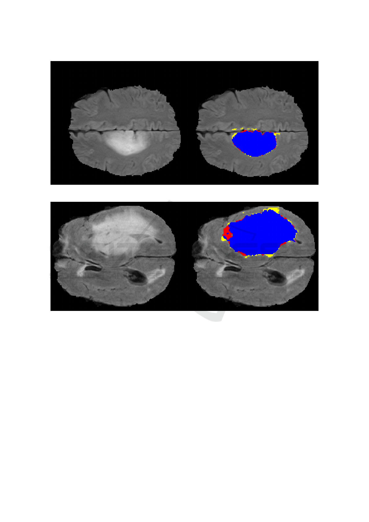
Figure 2: Segmentation example, case “pat466”, DSC 95%.
Figure 3: Segmentation example, case “pat254”, DSC 93%.
parison with our method is not possible, since the
hardware used was different, it is worth noting the rel-
atively small computational time of our method. Re-
duced run time is a valuable feature that should be
pursued, but without forgetting to take into account
the trade-off between computation time and segmen-
tation quality, which is an important part of the pro-
cess of designing a segmentation algorithm for CAD
systems (Menze et al., 2015).
Our implementation of the genetic algorithm clus-
tering method presents some differences from the
original. Through our tests, it was observed that us-
ing a population of 10 individuals and two to five
groups is sufficient to separate the pixels for the initial
segmentation. Also, selecting between the minimum
values of the clusters with higher mean intensities as
threshold produces higher DSC values, as it allows
for more flexibility in the thresholding operation. In
comparison, (Kole and Halder, 2012) used 30 indi-
viduals, selected tumor pixels from the cluster with
highest mean intensity, and empirically selected the
maximum number of groups for each image.
The percentage used for comparison between the
tumor and brain area was found empirically. This
comparison, together with the selection of the largest
connected component, is useful in eliminating “false
positives” that are created by tissues in the brain that
present themselves in the original FLAIR image as
high intensity regions, even though they are healthy.
In most cases, the AdaBoost classifier increased
the quality of the segmentation, improving, on aver-
age, the DSC in about 10%. The choice of features
– intensity and position in the slice – takes advan-
tage of the fact that, while different tumor structures
Brain Tumor Segmentation in Magnetic Resonance Images using Genetic Algorithm Clustering and AdaBoost Classifier
81

may present themselves with different intensity val-
ues, they are formed by contiguous regions of tissue,
and their position in consecutive slices do not deviate
much. However, the internal boundaries between tu-
mor tissues and the external boundaries between tu-
mor and healthy tissue, where tissue intensity may
change abruptly, might be a source of error. Including
adequate texture features, for example, may improve
overall performance.
One limitation to our study is the relatively small
number of images available to evaluate the technique,
although it is common practice in the literature to use
small private datasets to evaluate segmentation meth-
ods (Menze et al., 2015). Using more images would
provide a clearer picture of the proposed algorithm’s
performance and areas for improvement. Another
limitation is that the proposed technique heavily re-
lies on pixel intensity information, which is subject to
inter and intra slice variations caused by inhomogene-
ity in the magnetic resonance imaging field (Emblem
et al., 2009).
5 CONCLUSION
In conclusion, the method proposed in this paper com-
bines a genetic algorithm-based clustering method
with filters, morphological operation and an Ad-
aBoost classifier to automatically isolate the tumor
in magnetic resonance images. For the genetic algo-
rithm, improvements were achieved in comparison to
the original version: use of smaller population and a
fixed, small number of groups to perform the cluster-
ing, which allows for less computational effort. An-
other difference is the strategy that makes use of the
groups with highest and 2nd-highest mean intensi-
ties, allowing for adaptive restriction in the initial seg-
mentation. Additionally, the AdaBoost classifier im-
proved segmentation results by taking advantage of
both spatial and intensity information.
Future work may focus on improving the accu-
racy of this technique, by adapting it to evaluate and
include information from other magnetic resonance
modalities, such as T1-weighted. Also, the algorithm
can be further developed by adding methods to ana-
lyze texture features and better tuning of its numerical
parameters, such as the percentage of area for com-
parison between brain and tumor tissue and the num-
ber of rounds used to train the AdaBoost classifier.
Another option is to combine it with other machine-
learning techniques, such as support vector machines,
and create a segmentation based on the consensus of
two or more classification methods.
ACKNOWLEDGEMENTS
The authors would like to thank the support by grants
from São Paulo Research Foundation (FAPESP),
Brazilian Federal Agency for Support and Evalu-
ation of Graduate Education (Capes) and National
Council for Scientific and Technological Develop-
ment (CNPq).
REFERENCES
Alpaydin, E. (2014). Introduction to machine learning.
MIT press.
Emblem, K. E., Nedregaard, B., Hald, J. K., Nome, T.,
Due-Tonnessen, P., and Bjornerud, A. (2009). Auto-
matic glioma characterization from dynamic suscep-
tibility contrast imaging: Brain tumor segmentation
using knowledge-based fuzzy clustering. Journal of
Magnetic Resonance Imaging, 30(1):1–10.
Freund, Y. and Schapire, R. E. (1995). A desicion-theoretic
generalization of on-line learning and an application
to boosting. In European conference on computa-
tional learning theory, pages 23–37. Springer.
Gibbs, P., Buckley, D. L., Blackband, S. J., and Horsman,
A. (1996). Tumour volume determination from mr
images by morphological segmentation. Physics in
medicine and biology, 41(11):2437–2446.
Gordillo, N., Montseny, E., and Sobrevilla, P. (2013). State
of the art survey on mri brain tumor segmentation.
Magnetic resonance imaging, 31(8):1426–1438.
Johns Hopkins Medicine Health Library (2017). Gliomas.
[online] Hopkinsmedicine.org. Available at: https:
//goo.gl/8Ggjp8. [Accessed 15 Jul. 2017].
Kole, D. K. and Halder, A. (2012). Automatic brain tu-
mor detection and isolation of tumor cells from mri
images. International Journal of Computer Applica-
tions, 39(16):26–30.
Menze, B. H., Jakab, A., Bauer, S., Kalpathy-Cramer, J.,
Farahani, K., Kirby, J., Burren, Y., Porz, N., Slot-
boom, J., Wiest, R., et al. (2015). The multimodal
brain tumor image segmentation benchmark (brats).
IEEE transactions on medical imaging, 34(10):1993–
2024.
Schapire, R. E. (1999). A brief introduction to boosting. In
Ijcai, volume 99, pages 1401–1406.
Sonka, M., Hlavac, V., and Boyle, R. (2014). Image
processing, analysis, and machine vision. Cengage
Learning.
BIOIMAGING 2018 - 5th International Conference on Bioimaging
82
