
GPU Accelerated Probabilistic Latent Sequential Motifs for Activity
Analysis
Khaja Wasif Mohiuddin
1
, Jagannadan Varadarajan
1
, R
´
emi Emonet
3
, Jean-Marc Odobez
4
and Pierre Moulin
1,2
1
Advanced Digital Sciences Center, Singapore
2
Department of Electrical and Computer Engineering, University of Illinois at Urbana-Champaign, IL, U.S.A.
3
Jean Monnet University, Saint
´
Etienne, France
4
Idiap Research Institute, Martigny, Switzerland
Keywords:
PLSA, PLSM, Activity Analysis, Topic Models, GPU, CUDA, Motifs.
Abstract:
In this paper, we present an optimized GPU based implementation of Probabilistic Latent Sequential motifs
(PLSM) that was proposed for sequential pattern mining from video sequences. PLSM mines for recurrent
sequential patterns from documents given as word-time occurrences, and outputs a set of sequential activity
motifs and their starting occurrences. PLSM’s uniqueness comes from modeling the co-occurrence and tem-
poral order in which the words occur within a temporal window while also dealing with activities which occur
concurrently in the video. However, the expectation-maximization algorithm used in PLSM has a very high
time complexity due to complex nested loops, requiring several dimensionality reduction steps before invo-
king PLSM. In order to truly realize the benefits of the model, we propose two GPU based implementations
of PLSM called GPU-pLSM (sparse and dense). The two implementations differ based on whether the entire
word-count matrix (dense) or only the non-zero entries (sparse) are considered in inferring the latent mo-
tifs respectively. Our implementation achieves an impressive 265X and 366X times speed up for dense and
sparse approaches respectively on NVIDIA GeForce GTX Titan. This speed up enables us to remove several
pre-processing and dimension reduction steps used to generate the input temporal documents and thus apply
PLSM directly on the input documents. We validate our results through qualitative comparisons of the infer-
red motifs on two different publicly available datasets. Quantitative comparison on document reconstruction
based abnormality measure show that both GPU-PLSM and PLSA+PLSM are strongly correlated.
1 INTRODUCTION
We are entering an era of pervasive computing.
More and more private and public settings are equip-
ped with sensors such as proximity infrared sensors,
RFIDs, and CCTV cameras, generating tones of data
everyday. It is therefore, vital to create intelligent ma-
chines that can mimic human abilities; machines that
can observe colossal amounts of data and churn out
information with semantic significance and human in-
terpretability. Such information is useful in applicati-
ons such as surveillance, health care, infrastructure-
planning and human behaviour analysis. However,
the enormity of the generated data make even simple
learning algorithms several hours or even days to run.
Recently, the general purpose graphic processing
units (GPU) have become a powerful parallel compu-
ting platform, not only because of GPU’s multi-core
structure and high memory bandwidth, but also be-
cause of the popularity of parallel programming fra-
meworks such as CUDA that enable developers to ea-
sily manipulate GPU’s computing power. This mo-
tivates us to revisit and improvise conventional ma-
chine learning algorithms so that they can be used on
large-scale datasets.
Specifically, we consider the task of mining recur-
rent sequential patterns (called “motifs”) from large
scale videos collected from public spaces such as air-
ports, metro stations and shopping malls. Mining for
such patterns can be useful both in offline tasks such
as video summarization and understanding as well as
online tasks such as anomaly detection, where delays
in detection can cost dearly.
In this paper, we present accelerated imple-
mentations of Probabilstic Latent Sequential Motifs
(PLSM) (Varadarajan et al., 2010), a popular ap-
Mohiuddin, K., Varadarajan, J., Emonet, R., Odobez, J-M. and Moulin, P.
GPU Accelerated Probabilistic Latent Sequential Motifs for Activity Analysis.
DOI: 10.5220/0006537904090418
In Proceedings of the 13th International Joint Conference on Computer Vision, Imaging and Computer Graphics Theory and Applications (VISIGRAPP 2018) - Volume 5: VISAPP, pages
409-418
ISBN: 978-989-758-290-5
Copyright © 2018 by SCITEPRESS – Science and Technology Publications, Lda. All rights reserved
409

proach to discover sequential patterns from spatio-
temporal data. PLSM is topic model based approach
to activity mining in videos similar to probabilistic la-
tent semantic analysis (PLSA) (Hofmann, 2001) and
Latent Dirichlet Allocation (LDA) (Blei et al., 2003).
However, PLSM addresses the disadvantages of the
bag-of-words assumption in PLSA and performs tem-
poral modeling at multiple levels: a) within motifs to
identify when words occur, i.e., at which relative time
with respect to the motif beginning; b) within video
segments (temporal documents), to identify when a
motif actually starts in the document (more details in
sec 3.1). There are several advantages of temporal
modeling in PLSM: a) PLSM helps in understanding
how an activity unfolds over time enabling a time sen-
sitive visualization of the discovered activity patterns;
and b) it enables to precisely identify when an acti-
vity begins in a video, which could be used for tasks
including event counting. Furthermore, PLSM relies
on elegant generative model approach combined with
well established inference techniques to uncover the
latent variables. This allows an intuitive semantic in-
terpretation of the observed and latent variables, ma-
king it an easy choice despite a few recent deep lear-
ning based approaches towards activity analysis pre-
sented in (Xu et al., 2015; Hasan et al., 2016).
Earlier PLSM implementations (Varadarajan
et al., 2010) make use of complex dimensionality
reduction steps using LDA (Blei et al., 2003),
PLSA (Hofmann, 2001) to bring down the vocabu-
lary size and thereby the running time of PLSM, but
this is also cumbersome and time consuming. For
instance, it takes nearly 4.5 hours to apply PLSA on a
90 minute long video. While this reduces the running
time of PLSM, it is still inefficient due to the time
spent in other pre-processing steps. Furthermore, the
additional pre-processing layers also introduce diffi-
culties in motif visualization and in higher level tasks
such as abnormal event detection. Using multiple
pre-processing steps makes it difficult to reason out
which low-level feature caused an anomalous event.
On the other had, applying PLSM directly on videos
is complex and time taking due to high dimensional
nature of videos combined with complex nested
loops in PLSM EM procedure. However, thanks to
the cheap availability of GPUs these days, it is easier
to realize PLSM directly on the low-level visual
features, while still achieving superior running time
performance.
In this paper, we propose two different GPU based
implementations of PLSM i) Dense GPU-PLSM, ii)
Sparse GPU-PLSM. We perform the entire evaluation
on GPU in an efficient manner minimizing the data
transfers and providing good performance with high
Visual Words
(location, motion)
Video
bg. sub
optical flow
TSLA patterns
(pLSM words)
plsa on temporal window
connected comp.
pLSM
(sequencial motifs)
pLSM
Figure 1: Flowchart for discovering sequential activity mo-
tifs from videos using PLSM, as presented in (Varadarajan
et al., 2010).
scalability. In order to ensure that our implementa-
tion is scalable, we ran exhaustive set of experiments
using different generations of GPUs with increasing
number of cores and memory, while varying the in-
put dimensionality. We achieve peak performance of
nearly 265X using dense approach and 366X using
sparse approach.
2 RELATED WORK
Motion and appearance features have been used for
video based activity analysis for several years. For
instance, several methods have been proposed to (Xi-
ang and Gong, 2008; Li et al., 2008; Wang et al.,
2009) to fetch semantic activity patterns using low le-
vel features.
Recently, topic models like pLSA (Hofmann,
2001) LDA (Blei et al., 2003) originally proposed for
text processing have been successfully used with sim-
ple image features to discover scene level activity pat-
terns and detect abnormal events (Varadarajan and
Odobez, 2009; Li et al., 2008; Wang et al., 2009).
These Bag of Words methods assume that words are
exchangeable and their co-occurrence is sufficient to
capture latent patterns in the data. Using topic models
like pLSA allows the use of different abnormality me-
asures based on the interpretation of the model (Vara-
darajan and Odobez, 2009; Emonet et al., 2011). Ge-
nerative topic models for large set of documents with
large vocabulary size tend to consume too much com-
putation time. There have been efforts to speed up
probabilistic models like PLSA. For instance, Hong
et.al (Hong et al., 2008) proposed a CPU-based pa-
rallel algorithm for PLSA and made 6x speedup on
8-core CPU machines. Yu et. al. applied GPU in
Gibbs sampling for motif finding and achieved 10x
speedup (Yu and Xu, 2009). Yan et. al. proposed a
parallel inference method for Latent Dirichlet Alloca-
tion (LDA) on GPU and achieved 20x speedup (Yan
et al., 2009). However, there has been no such effi-
cient implementations for topic models that are po-
pular for video based activity analysis. Therefore, in
this paper, we consider the PLSM model that can be
applied on video data and propose two different GPU
implementations.
VISAPP 2018 - International Conference on Computer Vision Theory and Applications
410

p(ts|z,d)
p(z|d)
n(w, ta, d)
w
p(w,tr|z=1)
w
tr
p(w,tr|z=2)
w
tr
ta
z
ta
1
TdTd-Tr+1
8 11
(a)
d
z
t
a
t
s
t
r
w
D
Nd
(b)
Figure 2: Generative process as presented in (Varadara-
jan et al., 2010) (a) Illustration of the document n(w,t
a
,d)
generation. Words (w,t
a
= t
s
+t
r
) are obtained by first sam-
pling the topics and their starting times from the P(z|d) and
P(t
s
|z,d) distributions and then sampling the word and its
temporal occurrence within the topic from P(w,t
r
|z). (b)
Graphical model.
3 PLSM - PROBABILISTIC
LATENT SEQUENTIAL MOTIF
MODEL
In this section, we first introduce the notations and
provide an overview of the model, and then describe
with more details the generative process and the EM
steps derived to infer the parameters of the model.
PLSM describes the starting times of motifs within
a document as well as the temporal order in which
words occur within a motif.
Figure 2a showcases generation of documents.
Let D be the number of documents
1
d in the cor-
pus, each spanning T
d
discrete time steps. Let V =
{W
i
}
N
w
i=1
be the vocabulary of words that can occur
at any given instant t
a
= 1,..T
d
. A document is then
1
We use the terms topic and motifs interchangeably. Si-
milarly, we use the term document to refer to a video clip.
described by its count matrix n(w, t
a
,d) indicating the
number of times a word w occurs at the absolute time
ta within the document. These documents are genera-
ted from a set of N
z
topics {Z
i
}
N
z
i=1
assumed to be tem-
poral patterns P(w,t
r
|z) with a fixed maximal duration
of T
z
time steps (i.e. 0 ≤ tr< T
z
), where t
r
denotes the
relative time at which a word occurs within a topic,
and that can start at any time instant t
s
within the do-
cument. In other words, qualitatively, documents are
generated in a probabilistic way by taking the topic
patterns and reproducing them at their starting positi-
ons within the document, as illustrated in Figure 2a.
Figure 2a illustrates how documents are genera-
ted in our approach. Let D be the number of do-
cuments d in the corpus, each having N
d
words and
spanning T
d
discrete time steps . Let V = {w
i
}
N
w
i=1
be
the vocabulary of words that can occur at any given
instant t
a
= 1, ..T
d
. A document is then described by
its count matrix n(w,t
a
,d) indicating the number of
times a word w occurs at the absolute time t
a
within
the document. These documents are generated from
a set of N
z
topics {z
i
}
N
z
i=1
assumed to be temporal pat-
terns P(w,t
r
|z) with a fixed maximal duration of T
z
time steps (i.e. 0 ≤ t
r
< T
z
), where t
r
denotes the re-
lative time at which a word occurs within a topic, and
that can start at any time instant t
s
within the docu-
ment.
In other words, qualitatively, documents are gene-
rated in a probabilistic way by taking the topic pat-
terns and reproducing them at their starting positions
within the document, as illustrated in Fig.2a.
3.1 Generative Process
The actual process to generate all triplets (w,t
a
,d)
which are counted in the frequency matrix n(w,t
a
,d)
is given by the graphical model depicted in Figure 2b
and works as follows:
• draw a document d with probability P(d);
• draw a latent topic z ∼ P(z|d), where P(z|d) de-
notes the probability that a word in document d
originates from topic z;
• draw the starting time t
s
∼ P(t
s
|z,d), where
P(t
s
|z,d) denotes the probability that the topic z
starts at time t
s
within the document d;
• draw a word w ∼ P(w|z), where P(w|z) denotes
the probability that a particular word w occurs
within the topic z;
• draw the relative time t
r
∼ P(t
r
|w,z), where
P(t
r
|w,z) denotes the probability that the word w
within the topic z occurs at time t
r
;
• set t
a
= t
s
+ t
r
, which assumes that
P(t
a
|t
s
,t
r
) = δ(t
a
− (t
s
+ t
r
)), that is, the pro-
bability density function P(t
a
|t
s
,t
r
) is a Dirac
GPU Accelerated Probabilistic Latent Sequential Motifs for Activity Analysis
411

function. Alternatively, we could have modeled
P(t
a
|t
s
,t
r
) as a noise process specifying uncer-
tainty on the time occurrence of the word.
The joint distribution of all variables can be deri-
ved from the graphical model. However, given the
deterministic relation between the three time varia-
bles (t
a
= t
s
+ t
r
), only two of them are actually nee-
ded to specify this distribution (for instance, we have
P(w,t
a
,d,z,t
s
,t
r
) = P(t
r
|w,t
a
,d,z,t
s
)P(w,t
a
,d,z,t
s
) =
P(w,t
a
,d,z,t
s
) if t
a
= t
s
+ t
r
, and 0 otherwise). In
the following, we will mainly use t
s
and t
a
for con-
venience. In practice, we allow the motifs to start
anytime between 1 to T
ds
time steps, where T
ds
=
T
d
− T
z
+ 1. Accordingly, the joint distribution is gi-
ven by:
P(w,t
a
,d,z,t
s
) = P(d)P(z|d)P(t
s
|z,d)
P(w|z)P(t
a
−t
s
|w,z) (1)
Our final goal is to discover the topics and their
starting times given the set of documents n(w,t
a
,d).
This is a difficult task since the topic occurrences in
the documents overlap temporally, as illustrated in
Figure2a. The estimation of the model parameters Θ
can be done by maximizing the log-likelihood of the
observed data D, which is obtained through margi-
nalization over the hidden variables Y = {t
s
,z} (since
t
r
= t
a
−t
s
, see discussion above):
L(D|Θ) =
D
∑
d=1
N
w
∑
w=1
T
d
∑
t
a
=1
n(w,t
a
,d)
log
N
z
∑
z=1
T
ds
∑
t
s
=1
P(w,t
a
,d,z,t
s
) (2)
The above equation can not be solved directly due
to the summation terms inside the log. Thus, we
employ an Expectation-Maximization (EM) approach
and maximize the expectation of the complete log-
likelihood instead, which is given by:
E[L ] =
D
∑
d=1
N
w
∑
w=1
T
d
∑
t
a
=1
N
z
∑
z=1
T
ds
∑
t
s
=1
n(w,t
a
,d)
P(z,t
s
|w,t
a
,d)log P(w,t
a
,d,z,t
s
) (3)
with
P(z,t
s
|w,t
a
,d) =
P(w,t
a
d,z,t
s
)
P(w,t
a
,d)
(4)
and
P(w,t
a
,d) =
N
z
∑
z=1
T
ds
∑
t
s
=1
P(w,t
a
,d,z,t
s
) (5)
In the E-step, the posterior distribution of hidden
variables is then calculated as: where the joint pro-
bability is given by Eq. 1. Then, in the M-step, the
model parameters (the probability tables) are updated
according to (using the most convenient time varia-
bles, see end of Section 3.1):
P(z|d) ∝
T
ds
∑
t
s
=1
T
z
−1
∑
t
r
=0
N
w
∑
w=1
n(w,t
s
+t
r
,d)P(z,t
s
|w,t
s
+t
r
,d)
(6)
P(t
s
|z,d) ∝
N
w
∑
w=1
T
z
−1
∑
t
r
=0
n(w,t
s
+t
r
,d)P(z,t
s
|w,t
s
+t
r
,d)
(7)
P
w
(w|z) ∝
D
∑
d=1
T
ds
∑
t
s
=1
T
z
−1
∑
t
r
=0
n(w,t
s
+t
r
,d)P(z,t
s
|w,t
s
+t
r
,d)
(8)
P
t
r
(t
r
|w,z) ∝
D
∑
d=1
T
ds
∑
t
s
=1
n(w,t
s
+t
r
,d)P(z,t
s
|w,t
s
+t
r
,d)
(9)
In practice, the EM algorithm is initialized using
random values for the model parameters and stopped
when the data log-likelihood increase is too small. A
closer look at the above equations shows that qualita-
tively, in the E-step, the responsibilities of the topic
occurrences in explaining the word pairs (w,t
a
) are
computed (where high responsibilities will be obtai-
ned for informative words, i.e. words appearing in
only one topic and at a specific time), whereas the
M-steps aggregates these responsibilities to infer the
topic occurrences and the topic patterns. It is impor-
tant to notice that thanks to the E-steps, the multiple
occurrences of an activity in documents are implicitly
aligned in order to learn its pattern.
Once the topics are learned, their time occurrences
in any new document (represented by P(z|d
new
) and
P(t
s
|z,d
new
)) can be inferred using the same EM al-
gorithm, but using only Eq. 6 and Eq. 7 in the M-step.
The flowchart in Figure 1 shows how PLSM is ap-
plied on real-life videos. In order to apply the PLSM
model on videos, we need to define the words w for-
ming its vocabulary. One possibility would be to de-
fine some quantized low-level motion features and use
these as our words. However, due to the complex-
ity of PLSM inference (cf.1, 3), typically a dimensi-
onality reduction step relying on PLSA is introduced.
The topics from PLSA are then directly used as words
PLSM, while the word counts are obtained by measu-
ring the amount of each PLSA topic present in the
temporal window.
VISAPP 2018 - International Conference on Computer Vision Theory and Applications
412

4 GPU PLSM
PLSM involves computation of likelihood and proba-
bilities of a topic occurring in each iteration, which
involves several iterations of computationally inten-
sive steps looping over the number of documents (D),
number of topics (N
z
), vocabulary size (N
w
), starting
time (T
ds
). The overall complexity per iteration may
be given by O(N
w
∗N
z
∗D∗T
ds
∗T
d
). Every iteration is
dependant on previous iterations’ results, eventually
leading to the model parameters. The algorithm ter-
minates when convergence is attained or (and) maxi-
mum number of iterations (N
itr
) is reached.
To ensure coalesced access of data, document ar-
ray, initialised arrays layout were designed to facili-
tate inner loops and effectively use shared memory.
We implement the CUDA-accelerated GPU-PLSM
algorithm, which can be divided into three distinct
stages of operation. We stored relevant variables on
device memory to minimise data transfers and avoid
any duplicate evaluations. We have taken two appro-
aches to solve this problem depending on the number
of non-zero word count in the input document.
4.1 Dense GPU-PLSM
4.1.1 Stage 1 P(w, t
a
, d, z, t
s
)
Computing the joint distribution P(w,t
a
,d,z,t
s
) is a key
step in PLSM for Expectation-Maximization (EM) to
eventually compute the complete log-likelihood. This
evaluation comprises of nested looping along D, N
z
,
N
w
, T
ds
and T
z
. For every GPU kernel a grid, block
size is decided before processing the data. A grid is
a collection of 2D/3D blocks which in turn is further
divided into 2D/3D set of threads which belong to a
particular block. Based on the GPU architecture we
have mapped N
w
, D onto Grid(x,y) respectively and
block threads would be mapped to T
ds
. We provide
each thread sufficient work to loop over ranged para-
meters T
z
, N
z
processing them sequentially. All words
generated by a topic starting at time t
s
occur within a
document; hence t
s
takes values between 1 and T
ds
,
where T
ds
= T
d
- T
z
+ 1. However, we can also as-
sume that topics are partially observed beginning or
end are missing the frequency matrix. We had to be
careful to avoid any race conditions. It can be seen
that multiple pairs of (t
s
,t
r
) would write to a single
t
d
(t
s
+t
r
-1). In order to avoid concurrent write we fixed
t
r
in every block and exploited parallelism over t
s
in
batches. We effectively used the shared memory fea-
ture of Pascal architecture by loading common acces-
sed variables by the block threads to reduce the global
clock cycles. We were able to achieve occupancy of
100% effectively using shared memory to maximise
the throughput.
Algorithm 1: Cuda Kernel for P(w,t
a
,d,z,t
s
).
1: B
idx
← Number of Documents (d) on BlockId x
2: B
idy
← CorpusLength (w) on BlockId y
3: T
idx
← Timestamp (T
ds
) on ThreadId x
4: t
r
← Topic window (T
r
)
5: z ← number of Topics (N
z
)
6: S
Pd
← P
d
[B
idx
]
7: for t
r
<T
z
do
8: S
Pwtad
= 0
9: for z<N
z
do
10: S
Pzd
← P
zd
[z,B
idx
]
11: S
Ptszd
← P
tszd
[T
idx
,z,B
idx
]
12: S
Pwz
← P
wz
[B
idy
,z]
13: S
Ptrwz
← P
trwz
[t
r
,B
idy
,z]
14: SyncThreads()
15: S
Pwtad
+ = S
Pd
∗S
Pzd
∗S
Ptszd
∗S
Pwz
∗S
Ptrwz
16: SyncThreads()
17: P
wtad
+ = S
Pwtad
4.1.2 Stage 2: P(t
s
|z,d
new
), P(z|d
new
)
This is the M-step, where topics are learned and their
time of occurrence are inferred. This step is computed
by looping over N
w
, T
z
, N
w
, D and it is additionally
looped over T
ds
to compute P(z|d
new
). N
z
and D are
mapped on the Grid(x,y). N
w
and T
z
are looped in
chunks of 16,16 along thread dimension x,y. Global
arrays P
d
,P
tszd
,P
zd
,P
wz
,P
trwz
are stored partially on
device’s shared memory S
Pd
,S
Ptszd
,S
Pzd
,S
Pwz
,S
Ptrwz
.
We are able to achieve occupancy of 75% using 40
registers.
4.1.3 Stage 3 P(t
r
|w,z), P(w|z)
This computation is done only during training by loo-
ping over T
z
, D, T
d
, N
w
, N
z
. The approach is similar to
that of P(t
s
|z,d) kernel. N
w
and N
z
are mapped onto
Grid(x,y). T
ds
is mapped on ThreadIdx. Sequential
looping is done over t
r
and D. P(w|z) is then compu-
ted by summing over t
r
loop. A similar approach is
taken as used for computing P
tszd
. We were able to
achieve occupancy of 75% using 40 registers.
4.2 Sparse GPU-PLSM
When a document n(w,t
a
,d) is generated there are a
number of words whose frequency count is 0 in the set
of given documents. Only non-zero indices contribute
towards the computation and can be identified while
reading the term document. The idea is to process
only these non zero indices and skip the rest of the
GPU Accelerated Probabilistic Latent Sequential Motifs for Activity Analysis
413
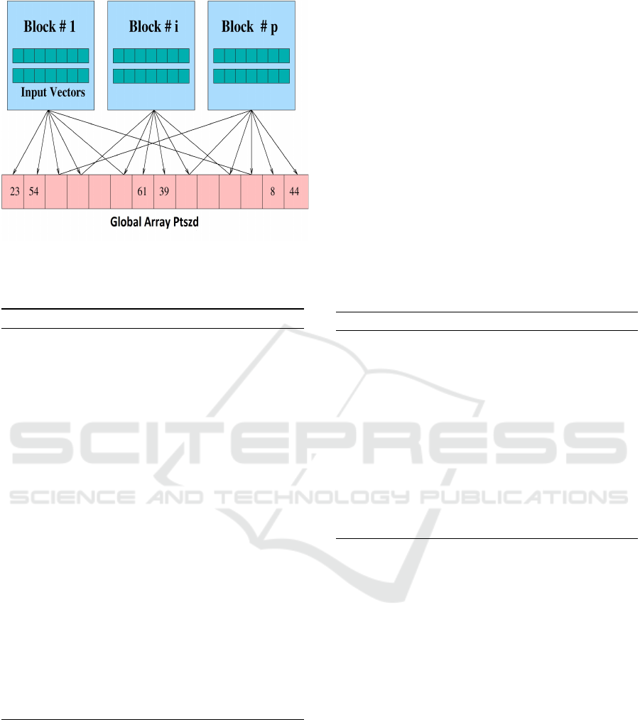
Figure 3: Layout of the CUDA blocks. Each block (128)
evaluates the document word count(w,t
a
,d) contribution to
P(t
s
|z,d) for possible values of T
s
,z.
Algorithm 2: Cuda Kernel for P(t
s
|z,d
new
) and P(z|d
new
).
1: B
idx
← number of Topics (N
z
) on BlockId x
2: B
idy
← Number of Documents (D) on BlockId y
3: T
idx
← CorpusLength (N
w
) on ThreadId x
4: T
idy
← Topic Window (T
z
) on ThreadId y
5: t
s
← Document Time window (T
ds
)
6: B
X
← Block Width
7: B
Y
← Block Height
8: S
Pd
← P
d
[B
idx
]
9: for t
s
<T
ds
do
10: S
Ptszd
= 0
11: S
Pzd
← P
zd
[B
idx
,B
idy
]
12: S
Ptszd
← P
tszd
[t
s
,B
idx
,B
idy
]
13: S
Pwz
← P
wz
[T
idx
,B
idx
]
14: S
Ptrwz
← P
trwz
[T
idy
,T
idx
,B
idx
]
15: w
i
d ← [T
idx
,t
s
+ T
idy
,B
idy
]
16: SyncThreads()
17: S
Ptszd
new
= S
Pd
∗ n[w
id
] ∗ S
Pzd
∗ S
Ptszd
∗ S
Pwz
∗
S
Ptrwz
/(Pwtad[w
id
] + epsilon)
18: for i=B
x
∗ B
y
/2,i>=1,i>>=1 do
19: S
tszd
new
[T
idx
]+ = S
tszd
new
[T
idx
+ i]
20: SyncThreads()
21: P(t
s
|z,d
new
)+ = S
tszd
new
[0]
22: P(z|d
new
)+ = P
tszd
new
evaluation. For every non zero entry it can be mapped
to an entry in (w,t
a
,d) tuple. For every t
a
there will be
multiple pairs of (t
s
,t
r
). We process set of non zero
word count n(w,t
a
,d) in each CUDA block as shown
in Figure 3. Global array P(t
s
|z,d
new
) would get mul-
tiple contributions from various blocks giving rise to
concurrent writes. We made use of fast atomic opera-
tions to ensure values are updated appropriately.
We experimented by storing n(w,t
a
,d) contribu-
tion to P(w, T
d
,d,t
s
) for various possibilities of T
s
in
a larger array and then shrink the array in a serial
fashion to P(t
s
|z,d
new
). This proved to be costly in
terms of storage. It would not scale to the increasing
set of parameters. We do one time book keeping of all
possible pairs that exist for every value of t
d
. All these
possible t
s
are stored in a single array and accessed
based on t
d
of the word. This is significantly helpful
in P(t
s
|z,d) and P(t
r
|w,z) P
trwz
evaluation which con-
sume major chunk of computation load. The problem
comes in while updating the tuple (t
s
,z,d) where in
multiple words w and topic window T
r
write to same
global location. Partitioning all such collisions into
respective bins would not be load balanced and also
give rise to divergence of threads. In order to resolve
concurrent write issue we used fast atomic operation.
This way all such global locations which face concur-
rent write problem are updated sequentially avoiding
any loss of data.
Algorithm 3: Sparse GPU-PLSM.
1: T
idx
← Non zero index
2: T
idy
← Number of Topics nZ
3: T s
id
← Possible values of Ts for Tidx
4: B
X
← Block Width 64
5: S
Ptszd
= 0
6: S
Pzd
← P
zd
[idx]
7: S
Ptszd
← P
tszd
[T
idx
]
8: for t
s
<Ts
id
do
9: S
Ptszd
new
+ = S
Pd
∗ Doc[w
i
d] ∗ S
Pzd
∗ S
Ptszd
∗
S
Pwz
∗ S
Ptrwz
/(Pwtad[w
i
d] + epsilon)
10: atomicAdd(P(t
s
|z,d
new
),S
Ptszd
new
)
11: atomicAdd(P(z|d
new
),S
Ptszd
new
)
5 EXPERIMENTAL RESULTS
We evaluated the performance of our GPU implemen-
tation two GPUs with varying capacity: i) NVIDIA’s
GTX Titan X, and ii) Quadro K620. The sequential
implementation was run on Intel(R) Xeon(R) CPU
3.50GHz. NVIDIA’s GTX Titan X for GPU provi-
des 11 teraflops of FP32 performance, powered with
3072 CUDA cores. Pascal architecture enables shared
memory of 49152 bytes per block and L2 cache me-
mory of 3145728 bytes. Quadro K620 comes with
384 cores and 2GB of device memory. We initia-
lize the CUDA hardware, allocating the appropriate
host and device memory. We also took into account
the available device memory to avoid memory leak.
For a typical set of parameters N
itr
= 50, N
w
= 75,
D = 140, T
ds
= 100, N
z
= 25, T
z
= 15 it would require
a memory size of 200 MB. The sequential implemen-
tation by (Varadarajan et al., 2010) has been used as
VISAPP 2018 - International Conference on Computer Vision Theory and Applications
414
0 0.2 0.4
0.6
0.8 1 1.2
·10
4
400
600
800
T
d
Time (ms)
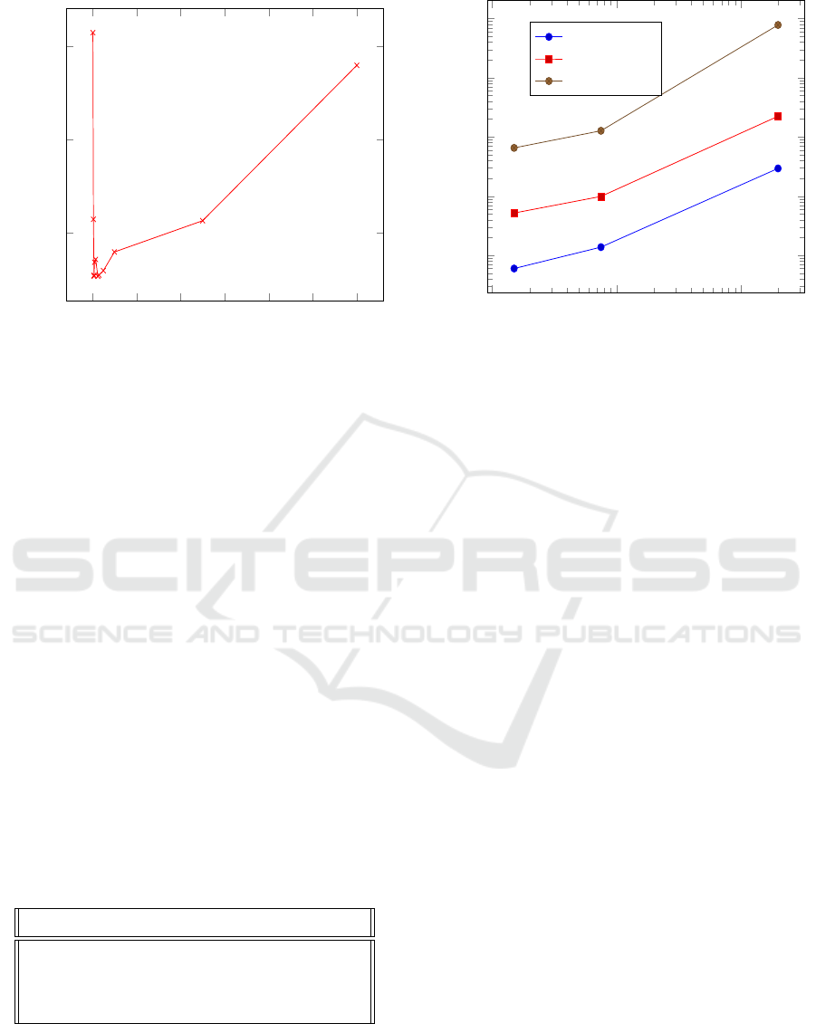
Figure 4: Run time performance of Dense-GPU implemen-
tation on GTX Titan X obtained by varying the document
length T
d
.
a benchmark to verify the accuracy of the parameters
and performance. The timings given in Table 1 are
average over 50 iterations of PLSM. Each iteration in-
cludes one complete EM step. We have performance
timing for vocabulary size upto 15000 and document
length of almost 2000. We evaluated the performance
by varying the vocabulary size N
w
, document length
T
d
and number of documents N
d
. Experiments were
carried out on low level features generated from ac-
tual surveillance video. We refer to (Varadarajan
et al., 2010) for details on how the low-level featu-
res are obtained. In the Dense-GPU approach, we
run through the complete document tuple n(w,t
a
,d)
to perform PLSM. We were able to exploit the GPU
architecture and reduce the computational complexity
from O(N
w
N
z
DT
ds
T
d
) to O (log(N
w
)N
z
T
s
).
The comparison of performance on CPU, GPU
have been done on actual video data. Table 1 shows
PLSM timings per iteration on CPU, Quadro K620
and GTX TitanX.
Table 1: Per iteration timings (ms) for PLSM with T
d
=100,
N
z
=25, T
z
=15.
Parameters(w,d) CPU K620 Titan
15,12 673 48.7 7.6
75,5 1298.9 97.3 13.12
75,140 47154.3 2479.3 334.1
1994,5 78545.3 2247 296.2
Figure 4 shows performance of the Dense-GPU
implementation obtained by varying the document
length T
d
. Since, the duration of the video is fixed,
increasing the document length will reduce the total
number of documents D. We observed the per itera-
10
1
10
2
10
3
10
1
10
2
10
3
10
4
10
5
N
w
Time (ms)
Titan
QuadroK620
CPU
Figure 5: Performance plot for PLSM per iteration against
Vocabulary size.
tion timing by varying document length from 25 to
11991 (actual document length) by fixing the number
of topics to N
z
= 25 and vocabulary size to N
w
= 75.
We found that best performance is obtained when T
d
is around 75. T
s
is mapped on to the block threads in
P
wtad
kernel, P
tszd
threads internally loop over T
s
. It is
clear that increasing T
d
would certainly increase the
computation load on P
tszd
kernel. Also since proces-
sing is done in warps, we observe an increase in the
throughput whenever T
s
is close to power of 2. So it
would be ideal to choose a T
s
value that is a power
of 2 that would also give rise to adequate number of
documents.
Figure 5 shows performance comparison of GPU-
PLSM against the CPU PLSM for varying size of the
vocabulary on GPU Titan X and Quadro K620. We
observed that with increasing vocabulary size perfor-
mance on Titan X saw a boost by giving a speedup of
145X. The number of cores scale well with increasing
N
w
. The scalability in the number of cores of the GPU
can be seen on low end card like Quadro K620 with
384 cores and device memory (2 GB). So in this we
have limited our vocabulary size and compared the in-
dividual performance of K620 (peak performance 863
GFLOPS) with that of TitanX (peak performance of
1TB). For low input size, the performance of K620
compared to other high end card is shown in Figure 5.
GTX Titan boosted the speed on an average by a fac-
tor of 7.6 compared to Quadro K620. The significant
points are that the Quadro K620 also was able to give
good performance and the algorithm scales well with
increasing number of cores.
Figure 6 shows comparison of sparse and dense
implementation of GPU-PLSM on Titan X for vari-
ous values of N
w
, i.e., vocabulary size. For small N
w
,
GPU Accelerated Probabilistic Latent Sequential Motifs for Activity Analysis
415
10
1
10
2
10
3
10
1
10
2
10
3
10
4
N
w
Time (ms)
Dense
Sparse
Figure 6: Performance plot for Sparse and Dense GPU-
PLSM per iteration on GTX Titan.
the sparse implementation does well providing 2.3 ti-
mes speedup compared to the usual dense approach.
But for larger values of N
w
the dense approach perfor-
mance better than the sparse approach. The main re-
ason behind this counter-intuitive behaviour for large
N
w
is the large number of collisions in the atomicAdd
operation while updating the global variables. Howe-
ver, one could chose either of the implementations ba-
sed on the input parameters and number of non-zero
entries in the document.
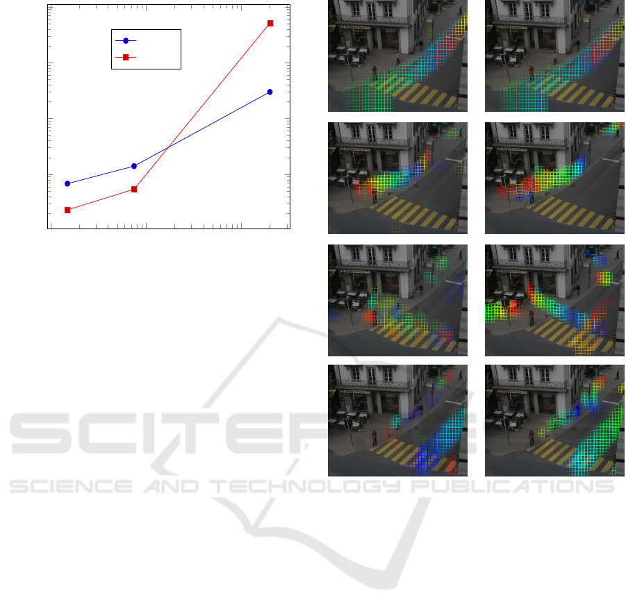
5.1 Visualization
The Traffic Junction video (see Figure 7) is 45 mi-
nutes long and captures a portion of a busy traffic-
light-controlled road junction. Typical activities in-
clude people walking on the pavement or waiting be-
fore crossing over the zebras, and vehicles moving in
and out of the scene. The data set videos have a frame
size of 280 × 360.
The first column (Figure 7a) shows visual re-
sults using PLSA+PLSM and the second column (Fi-
gure 7b) shows results from our GPU-PLSM. The
discovered patterns are superimposed on the scene
image, where the colors represent the relative time
from the start of the activity, i.e., violet indicates the
first time step and red indicates the last time step of
the activity. We can observe that results from PLSA-
PLSM and GPU-PLSM are indeed quite similar in-
dicating that there is no loss in the output of GPU-
PLSM when low level features are directly fed to the
model.
The Far Field video from (Varadarajan et al.,
2010) (see Fig. 8) contains 108 minutes of a three-
(a) (b)
Figure 7: Traffic Junction a) Sequential Motif using
PLSA,PLSM b) Sequential Motif using only GPU-PLSM
on low level features. Colors represent the relative time
from the start of the activity, i.e., violet indicates the first
time step and red indicates the last time step of the activity.
road junction captured from a distance, where typi-
cal activities are moving vehicles. As the scene is not
controlled by a traffic signal, activities have large tem-
poral variations. For this event detection task, we la-
belled a 108 minute video clip from the far field scene,
distinct from the training set Figure 8a shows visual
results obtained using PLSA+PLSM as done in (Va-
radarajan et al., 2010), and Figure 8b shows results
obtained using GPU-PLSM. We can observe from the
visualization that the results from both the implemen-
tations are comparable.
5.2 Abnormality Measure
We also compared the two approaches quantitatively,
to validate our GPU based implementations. For this
we used the mean absolute document reconstruction
error (MADRE) proposed by ((Emonet and Odobez,
VISAPP 2018 - International Conference on Computer Vision Theory and Applications
416
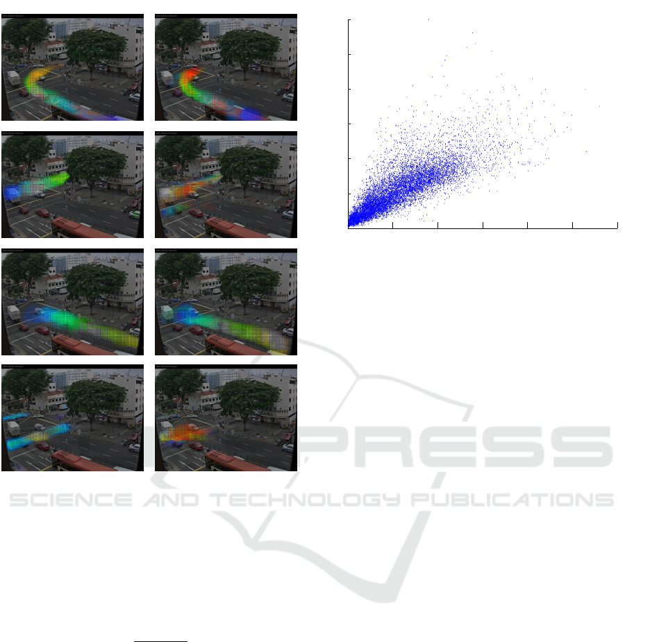
(a) (b)
Figure 8: Far Field a) Sequential Motif using PLSA+PLSM
b) Sequential Motif using GPU-PLSM directly on the low
level features.
2012)). More precisely, given the observed word-
count matrix n(w,t
a
,d), and the reconstructed (recon-
structed via inference) document word-count matrix
P(w,t
a
|d), the abnormality measure is defined as:
MADRE(t
a
,d) =
∑
w
|
n(w,t
a
,d)
n(d)
− P(w,t
a
|d)| (10)
P(w,t
a
|d) =
∑
z
∑
ts
P(w,t
a
,d,z,t
s
) (11)
In order to compare the GPU-PLSM with PLSA-
PLSM, we show a scatter plot of the MADRE values
obtained by the two methods in Figure 9. From the
scatter plot, we find that the two methods exhibit a
strong correlation. In order to ensure that the detecti-
ons from the two methods will be the same, they need
to have a strong positive correlation. We observed
that the values obtained from the two methods have
a correlation coefficient of 0.7979 indicating a strong
positive linear relationship between them.
0 20 40 60 80 100 120
0
0.5
1
1.5
2
2.5
3
MADRE PLSA − PLSM
MADRE GPU−PLSM
Figure 9: Scatter plot using MADRE for PLSM against
PLSA+PLSM.
6 CONCLUSIONS
In this paper, we presented a GPU-PLSM approach
to address the running time inefficiencies found in
PLSM method used for video based activity analy-
sis applications. To this end, we proposed two va-
riants of the GPU-PLSM, namely, dense and sparse
GPU-PLSM, based on whether the non-zero entries
are used in the computation or not in the EM com-
putation respectively. Through experiments done on
two different GPU platforms, we were able to achieve
a top speed up of 366X compared to its CPU coun-
terpart. We further validated our results from GPU-
PLSM using both qualitative and quantitative compa-
risons and showed that the results from GPU-PLSM
correlate well with the vanilla PLSM implementation.
We believe that our contribution will encourage real
time analysis and detection of abnormal events from
videos. In future work, we plan to work more on opti-
mizing the sparse approach for large vocabulary sizes
to bring down the computation time and improve me-
mory optimization.
ACKNOWLEDGEMENTS
This study is supported by the research grant for
the Human Centered Cyber-physical Systems Pro-
gramme at the Advanced Digital Sciences Center
from Singapore's Agency for Science, Technology
and Research (A*STAR). The authors thank NVIDIA
for donating GPUs to support this research work.
GPU Accelerated Probabilistic Latent Sequential Motifs for Activity Analysis
417

REFERENCES
Blei, D. M., Ng, A. Y., and Jordan, M. I. (2003). Latent
dirichlet allocation. Journal of machine Learning re-
search, 3(Jan):993–1022.
Emonet, R. and Odobez, J.-M. (2012). Intelligent Video
Surveillance Systems (ISTE). Wiley-ISTE.
Emonet, R., Varadarajan, J., and Odobez, J. (2011). Multi-
camera open space human activity discovery for ano-
maly detection. In 8th IEEE International Conference
on Advanced Video and Signal-Based Surveillance,
AVSS, pages 218–223.
Hasan, M., Choi, J., Neumann, J., Roy-Chowdhury, A. K.,
and Davis, L. S. (2016). Learning temporal regularity
in video sequences. CoRR, abs/1604.04574.
Hofmann, T. (2001). Unsupervised learning by probability
latent semantic analysis. Machine Learning, 42:177–
196.
Hong, C., Chen, W., Zheng, W., Shan, J., Chen, Y., and
Zhang, Y. (2008). Parallelization and characterization
of probabilistic latent semantic analysis. In 2008 37th
International Conference on Parallel Processing, pa-
ges 628–635.
Li, J., Gong, S., and Xiang, T. (2008). Global behaviour
inference using probabilistic latent semantic analysis.
In British Machine Vision Conference.
Varadarajan, J., Emonet, R., and Odobez, J. (2010). Proba-
bilistic latent sequential motifs: Discovering tempo-
ral activity patterns in video scenes. In British Ma-
chine Vision Conference, BMVC 2010, Aberystwyth,
UK, August 31 - September 3, 2010. Proceedings, pa-
ges 1–11.
Varadarajan, J. and Odobez, J. (2009). Topic models for
scene analysis and abnormality detection. In ICCV-
12th International Workshop on Visual Surveillance.
Wang, X., Ma, X., and Grimson, E. L. (2009). Unsuper-
vised activity perception in crowded and complica-
ted scenes using hierarchical bayesian models. IEEE
Trans. on PAMI, 31(3):539–555.
Xiang, T. and Gong, S. (2008). Video behavior profiling for
anomaly detection. IEEE Trans. on PAMI, 30(5):893–
908.
Xu, D., Ricci, E., Yan, Y., Song, J., and Sebe, N. (2015).
Learning deep representations of appearance and mo-
tion for anomalous event detection. In Xianghua Xie,
M. W. J. and Tam, G. K. L., editors, Proceedings of
the British Machine Vision Conference (BMVC), pa-
ges 8.1–8.12. BMVA Press.
Yan, F., Xu, N., and Qi, Y. (2009). Parallel inference for la-
tent dirichlet allocation on graphics processing units.
In Bengio, Y., Schuurmans, D., Lafferty, J. D., Wil-
liams, C. K. I., and Culotta, A., editors, Advances
in Neural Information Processing Systems 22, pages
2134–2142. Curran Associates, Inc.
Yu, L. and Xu, Y. (2009). A parallel gibbs sampling algo-
rithm for motif finding on gpu. In 2009 IEEE Inter-
national Symposium on Parallel and Distributed Pro-
cessing with Applications, pages 555–558.
VISAPP 2018 - International Conference on Computer Vision Theory and Applications
418
