
Deep Parts Similarity Learning for Person Re-Identification
Mar
´
ıa Jos
´
e G
´
omez-Silva, Jos
´
e Mar
´
ıa Armingol and Arturo de la Escalera
Intelligent Systems Lab (LSI) Research Group,
Universidad Carlos III de Madrid, Legan
´
es, Madrid, Spain
Keywords:
Deep Learning, Convolutional Neural Network, Mahalanobis Distance, Person Re-Identification.
Abstract:
Measuring the appearance similarity in Person Re-Identification is a challenging task which not only requires
the selection of discriminative visual descriptors but also their optimal combination. This paper presents a
unified learning framework composed by Deep Convolutional Neural Networks to simultaneously and auto-
matically learn the most salient features for each one of nine different body parts and their best weighting to
form a person descriptor. Moreover, to cope with the cross-view variations, these have been coded in a Ma-
halanobis Matrix, in an adaptive process, also integrated into the learning framework, which takes advantage
of the discriminative information given by the dataset labels to analyse the data structure. The effectiveness
of the proposed approach, named Deep Parts Similarity Learning (DPSL), has been evaluated and compared
with other state-of-the-art approaches over the challenging PRID2011 dataset.
1 INTRODUCTION
Person re-identification (re-id) consists of recognizing
an individual through images from non-overlapping
camera views at different locations and time. Auto-
mating this task has become one of the major goals
in intelligent video-surveillance, since many other ap-
plications, like tracking or behaviour analysis, rely on
the person re-id performance. Usually, in real-world
surveillance scenarios, fine biometric cues are unavai-
lable, so the research has been mainly focused on the
appearance-based approaches.
The literature presents two re-id strategies: sin-
gle shot recognition, (Munaro et al., 2014), where
only one image per person and per view is used, and
multi-shot recognition, (Khan and Br
´
emond, 2016)
and (Chan-Lang et al., 2016), where a tracklet of
every individual (i.e. small sequence of images) is
available for each camera view. This paper is focu-
sed on the single-shot case, where the aim of the re-id
task is to identify the person represented by an image
from one view (probe image) among all the images
from the other view (gallery images).
The single-shot re-identification problem can be
treated as a pairwise binary classification, consisting
of two steps: the features extraction for pairs of ima-
ges and the learning of their optimal combination to
discriminate similar and dissimilar pairs.
The selection of features based on visual appea-
rance becomes a remarkable challenge in unconstrai-
ned scenarios, because of the inter-class ambiguities
and the intra-class variations. The first ones are pro-
duced by the similar appearances when different pe-
ople are wearing similar clothes or hairstyles, and the
second ones are due to the changes in resolution, il-
lumination, pose, perspective, background, etc. bet-
ween the two cameras views that cause extremely dif-
ferent representations of the same person.
In order to face this problem, two research streams
can be found: those which enhance the design of the
features, or the ones focused on improving the way
of combining them. The first group tries to represent
the most discriminant aspects of an individuals appea-
rance, advancing in the direction of extracting seman-
tically meaningful attributes (Layne et al., 2014).
On the other hand, the learning of a distance to
optimally combine some visual features can boost
the re-identification performance using quite simple
hand-crafted features, mainly based on colour or tex-
ture. Some methods address the distance learning
through evaluating the discriminative importance of
different types of features, as it is presented in (Liu
et al., 2014). Other methods are meant to learn a me-
tric that reflects the visual camera-to-camera transi-
tion, (Roth et al., 2014).
Most of these approaches optimize a linear
function to properly weight the absolute difference
between the images features of a pair, after that fe-
atures have been computed for a dataset, treating the
features selection and the distance learning as two in-
Gómez-Silva, M., Armingol, J. and Escalera, A.
Deep Parts Similarity Learning for Person Re-Identification.
DOI: 10.5220/0006539604190428
In Proceedings of the 13th International Joint Conference on Computer Vision, Imaging and Computer Graphics Theory and Applications (VISIGRAPP 2018) - Volume 5: VISAPP, pages
419-428
ISBN: 978-989-758-290-5
Copyright © 2018 by SCITEPRESS – Science and Technology Publications, Lda. All rights reserved
419

dependent stages. On the contrary, this paper pre-
sents a training framework were the features and their
combination are jointly learnt in a unified architec-
ture formed by Deep Convolutional Neural Networks
(DCNN). This proposal, hereinafter called Deep Parts
Similarity Learning (DPSL), presents the following
highlights:
1. The feature learning has been divided according
to nine body parts, to get more robustness against
partial occlusions. The features corresponding to
each body part are parallelly learnt in the same
process, getting a representation which is more
invariant to the pose and eliminating a huge part
of the background dependency. A body parts ex-
traction stage has been designed using a Convo-
lutional Pose Machine (CPM), (Wei et al., 2016),
which has been integrated into the learning frame-
work, leading to a highly-layered architecture.
2. The proper weighting of the learnt features has
been also addressed by the deep learning strategy,
allowing the automatic search of the most discri-
minative person descriptor. This is achieved by a
fully connected layer, whose inputs are the extrac-
ted features for every body part.
3. The intra-class variations are coped with a discri-
minative analysis of the data structure, which has
been encompassed in a Mahalanobis Matrix. The
Mahalanobis Matrix is employed to code the vi-
sual camera-to-camera transitions, and its estima-
tion has been optimized by the adaptively learning
of the covariance matrices of two features spaces,
the similar and dissimilar ones.
4. All the stages, body parts extraction, feature and
weighting learning, and data structure analysis,
are integrated into a unified learning framework.
The re-id capacity of the proposed approach has
been evaluated over one of the most challenging and
commonly used re-id datasets: PRID2011
1
(Hirzer
et al., 2011), using the standard protocols. The ex-
perimental results have proved the improvements in
comparison with other state-of-the-art methods.
The rest of the paper is organized as follows.
Section 2 presents the existing related work. The
proposed re-id learning framework is described in
Section 3. Section 4 evaluates the learning process
evolution and presents the experimental results, and
some concluding remarks are given in Section 5.
1
The dataset is publicly available under http://lrs.icg.
tugraz.at/download.php
2 RELATED WORK
With the aim of solving the re-id problem, many
works have been dedicated to the design of featu-
res able to represent the most discriminant aspects
of an individual's appearance. RGB or HSV histo-
grams (Bazzani et al., 2013), Gabor filters (Zhang and
Li, 2011) and HOG-based signatures (Oreifej et al.,
2010), are examples of descriptors based on low-level
local features, such as colour, texture, and shape re-
spectively.
Traditionally, many algorithms have used Princi-
pal Component Analysis (PCA) method to reduce the
dimensionality of the computed features, like in (Roth
et al., 2014). An alternative to the dimensionality re-
duction is the integration of several types of features
into a global signature, such as Bag-of-words (BoW)
models. In (Ma et al., 2014), BoW model is improved
by means of using the Fisher Vector, (S
´
anchez et al.,
2013), which encodes higher order statics of local fe-
atures.
To make the features invariant to pose and robust
against partial occlusions, region-based approaches
decompose the human shape in different articulated
parts and extract features for each one, like (Bazzani
et al., 2014), where a symmetry-based silhouette par-
tition is used to detect salient body regions. In (Cheng
and Cristani, 2014), a pose estimation stage, based on
Pictorial Structures, (Felzenszwalb and Huttenlocher,
2005), is presented, from which traditional features
are subsequently computed. Instead of that, this pa-
per proposes the integration of a Convolutional Pose
Machine (CPM), (Wei et al., 2016), into the learning
framework. In that way, spatial information is also
integrated into the feature representation.
In order to get only one metric value to measure
the similarity between two images, the matching is
performed by computing a certain distance between
the descriptors. In (Hirzer et al., 2012) the Euclidean
distance is used. However, recently, a large amount
of research has been focused on searching for the op-
timal metric. In that way, the features selection pro-
blem is addressed not only improving the descriptors
design but also the selection mechanism.
In (Liu et al., 2014), a Prototype-Sensitive Fea-
ture Importance based method is proposed to adap-
tively weigh the features according to different clus-
ters of population, instead of using a Global Feature
Importance (GFI) measure. This last approach is wi-
dely extended and assumes a global weighting, i.e.
a vector of generic weights and invariant to the po-
pulation. Some examples are Boosting (Gray and
Tao, 2008), Ranking Support Vector Machines (Rank-
SVM), (Prosser et al., 2010), Probabilistic Relative
VISAPP 2018 - International Conference on Computer Vision Theory and Applications
420

Figure 1: DPSL architecture.
Distance Comparison (PRDC), (Zheng et al., 2011),
or Metric Learning algorithms, such as Linear Discri-
minant Analysis (LDA) (Fisher, 1936) and Logistic
Discriminant Metric Learning (LDML) (Guillaumin
et al., 2009).
Rank-SVM (Prosser et al., 2010) is used to le-
arn an independent weight for each feature. Instead
of that, Mahalanobis metric learning optimizes a full
matrix that relates all the features between each ot-
her, exploiting the structure of the data, under the as-
sumption that the classes present the same distribu-
tion. Therefore, this is employed in this work to code
the view-to-view transitions, so that, the cross-view
variations are reduced.
The Mahalanobis matrix estimation has been
made through an adaptive data analysis process inte-
grated into the features and weighting learning, which
affects on the learning evolution, improving it.
The recent boost of deep learning algorithms has
made possible the automatic search of salient high-
level representations from the pixels of an image by
means of training DCNNs like it is proposed in this
work. Concretely for the re-id task, the learning has
been commonly performed by Siamese Networks (Yi
et al., 2014), consisting of two DCNNs sharing pa-
rameters and joined in the last layer, where the loss
function leads the whole network to discriminate bet-
ween pairs of similar or dissimilar images.
3 DEEP PART SIMILARITY
LEARNING, DPSL
In this section, the DPSL framework is presented. A
general view of the architecture is given in the first
subsection. The rest of the subsections describe each
one of the stages, compounding it, in detail.
3.1 Architecture
To learn to identify the similarity between two per-
son images, a Siamese architecture is used. The Si-
amese network is formed by two branches (one per
person image) which are composed of a combination
of DCNN to learn the optimal person representation
for each person of a pair. The branches are joined in
the final layers, where the similarity is measured, by
means of comparing the obtained features. The whole
architecture is presented in Figure 1, which is explai-
ned below.
The input of each branch is one of the images, I
p
,
of the pair to compare, where the index p indicates
each one of the two branches, a, or, b.
Moreover, each image has an identity number,
ID(I
p
), to identify the person to whom the image be-
longs. The labeller layer is in charge of checking if
the pair is a positive one, when the represented person
is the same in both images (same identity numbers),
or a negative one, otherwise. Its output, y, takes value
1 for positive pairs, and 0, for negative ones.
Firstly, from each person image, nine different
body parts images,
bp
I
p
, are extracted. The index
bp indicates the query body part, taking the following
values: h, head; ula, upper left arm; lla, lower left
arm; ura, upper right arm; lra, lower right arm; ull,
upper left leg; lll, lower left leg; url, upper right left;
lrl, lower right leg.
Secondly, a DCNN computes a multi-dimensional
descriptor,
bp
F
p
, for each one of the mentioned parts.
Subsequently, the descriptors are weighted to com-
pose a feature array, F
p
, to represent each person
image. These representations are analysed in every
iteration to get an estimation of the Mahalanobis Ma-
trix, M, in the Data Structure Analysis stage, where
the discriminative information given by the label y is
also considered.
Deep Parts Similarity Learning for Person Re-Identification
421
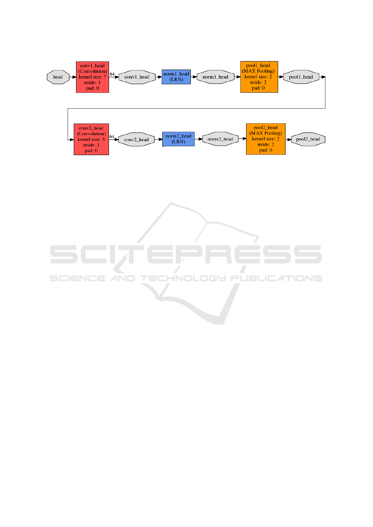
Figure 2: DCNN used to learn the head feature matrix,
h
F
p
.
Then, in the connection layer, the Mahalanobis
distance is computed and its value is taken as a dis-
tance metric, dm, to measure the dissimilarity bet-
ween the feature arrays.
Finally, the loss function measures the deviation
of the distance value with respect to the established
objective values for positive and negative pairs. The
loss value determines the evolution of the whole lear-
ning process by means of the forward and back pro-
pagation method (Rumelhart et al., 1988).
3.2 Body Parts Extractor
The body parts extractor layer takes as input a person
image, I
p
, and returns nine body parts images,
bp
I
p
,
whose sizes have been pre-established according to
the human shape proportions applied to a human re-
presentation with a height of 128-pixels, which is the
height value presented by the samples in most of the
re-identification datasets. Eventually, the established
body part sizes are 45x45, for
h
I
p
, 30x40 for
ula
I
p
,
lla
I
p
,
ura
I
p
, and
lra
I
p
, and 30x60 for
ull
I
p
,
lll
I
p
,
url
I
p
,
and
lrl
I
p
.
This body parts extractor layer is mainly based on
the CPM presented in (Wei et al., 2016), whose out-
puts are a set of body joints locations.
For each body part a Region Of Interest, ROI,
which is defined by a rotated rectangle, is extracted
from the input image. The orientation angle of the
rectangle is the one presented by the line resulting
of joining the extreme joints of the query body part.
The location of the upper joint is chosen as the upper
central pixel of the ROI and the location of the lower
joint, as its lower central pixel.
3.3 Deep Convolutional Neural
Network, DCNN
For each body part image,
bp
I
p
, a DCNN is used to
learn the corresponding part feature,
bp
F
p
, which is a
multi-dimensional descriptor. This can be understood
as a matrix whose elements are vectors with a length
value of 64. The resulting matrix dimensions are 8x8
for
h
F
p
, 7x4 for
ula
F
p
,
lla
F
p
,
ura
F
p
, and
lra
F
p
, and
12x4 for
ull
F
p
,
lll
F
p
,
url
F
p
, and
lrl
F
p
.
Even, the weights and dimensions of these nine
types of networks are different, they present an iden-
tical structure. As an example, Figure 2 presents the
DCNN corresponding to the head, essentially formed
by two types of layers: convolutional (in red) and
max-pooling (in yellow) layers, using a rectified li-
near unit (ReLU) as activation function. This neural
network architecture is based on the first layers con-
figuration of the mnistsiamese example, implemented
by the Caffe libraries (Jia et al., 2014), which presents
a traditional CNN architecture.
The nine DCNN have been duplicated sharing the
same weights, so the learnt descriptors are the same in
both branches, which is the base of a Siamese Neural
Network training.
3.4 Weighting
Once each part feature,
bp
F
p
, has been computed, the
optimal weighting is learnt, using an inner product
layer, which is a fully connected layer, that weighs
and combines all the part features to create the ele-
ments of a general person descriptor, F
p
, whose size,
N(N = 100)has been experimentally fixed.
However, the inputs of the inner product must be
the elements of a single matrix, so a first stage of con-
catenation is needed to form it from the parts features
VISAPP 2018 - International Conference on Computer Vision Theory and Applications
422
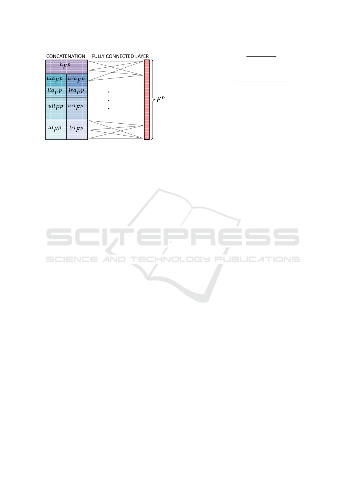
Figure 3: Creation of the Person Feature array, F
p
.
matrices, resulting in a 46x8 matrix as the Figure 3
describes.
3.5 Labeller
Throughout the learning process every input image, I,
is accompanied by an Identification Number, ID(I).
With the aim of knowing if the computed features, F
a
s
and F
b
s
, represent a positive or a negative pair of ima-
ges, the labeller function, y(F
a
s
, F
b
s
), takes the values
1 or 0 according to (1).
y(F
a
s
, F
b
s
)
1 ID(I
a
s
) = ID(I
b
s
)
0 ID(I
a
s
) 6= ID(I
b
s
)
(1)
3.6 Connection Function
Once the person representation, F
p
, has been com-
puted for each one of the images of an input pair,
they must be compared by the connection function,
f
cn
(F
a
, F
b
), in order to get the distance metric, dm,
that measures the dissimilarity between the images.
The connection function, f
n
(F
a
, F
b
), takes two
different formulations along the learning process, as
(2) shows, so the comparison of features is made by
the Euclidean distance, d
E
, until the number of le-
arning iterations, it, achieves a certain threshold, T
it
,
then, the comparison is made by the Mahalanobis dis-
tance, d
M
, instead.
The Euclidean distance between the descriptors,
d
E
(F
a
, F
b
), is defined by (3), where f
p
n
renders each
element of a person descriptor, F
p
.
The Mahalanobis distance, d
M
(F
a
, F
b
), is defined
by (4), where M is the Mahalanobis Matrix. This can
be understood as the inverse matrix of the covariance
matrix for the variable formed by the difference of our
feature arrays, F
a
− F
b
.
dm = f
c
(F
a
, F
b
) =
d
E
(F
a
, F
b
) it < T
it
d
M
(F
a
, F
b
) it ≥ T
it
(2)
d
E
(F
a
, F
b
) =
s
N
∑
n=1
( f
a
n
− f
b
n
) (3)
d
M
(F
a
, F
b
) =
q
(F
a
− F
b
)
T
M(F
a
− F
b
) (4)
Therefore, M allows us to consider the data struc-
ture for that new array, F
a
− F
b
, encoding the relati-
onship of each one of its elements with each other, as
it is described in Section 3.7.
However, a reliable estimation for the Mahalano-
bis Matrix is not achieved until executing an experi-
mentally observed number of learning iterations, T
it
.
For that reason the Euclidean distance is employed in
the first stage of the learning process.
3.7 Discriminative Data Structure
Analysis
The objective of this module is to estimate the Ma-
halanobis matrix that the connection function needs
by means of analysing the probabilistic distribution
of the variable formed by the difference between the
computed features, F
a
s
− F
b
s
, and discriminating if
they belong to positive or negative samples, thanks
to the information given by the labeller function, y.
In every iteration of the DPSL, the input is not
only a single pair of images but a batch of them. The-
refore, the input of this module is a Batch of Pairs of
features BoP, defined by (5), where B is the batch size
(B = 128).
BoP = {P
s
: P
s
= (F
a
s
, F
b
s
) ∀s ∈ [1, B]}. (5)
Subsequently, the BoP is divided into two subsets:
the similarity set, S, and the dissimilarity set, D, defi-
ned by (6) and (7) respectively.
S = {|F
a
s
− F
b
s
| | y(F
a
s
, F
b
s
) = 1 ∧ s ∈ [1, B]}. (6)
D = {|F
a
s
− F
b
s
| | y(F
a
s
, F
b
s
) = 0 ∧ s ∈ [1, B]}. (7)
We call SQ to a FIFO (First In, First Out) queue of
size K(K = 1000) where the elements of the subset S,
are added in every iteration, and, in the same way, DQ
to a queue of size K that accumulates the elements of
the subset D.
Therefore, these queues are KxN matrices, since
N is the dimension of the features arrays and con-
sequently the dimension of their difference vector,
F
a
s
− F
b
s
. When the queues are full, the firstly added
elements are deleted to continue adding new ones in
Deep Parts Similarity Learning for Person Re-Identification
423

order to consider the effects of the most recent trai-
ning samples on the Mahalanobis Matrix, M, learning
in every iteration.
SQ and DQ represent a subset of the difference
feature space for the situation of similarity (positive
pairs) or dissimilarity (negative pairs), so they are
used to computed the similarity covariance matrix,
Σ
S
, and the dissimilarity covariance matrix, Σ
D
, as it
is described by (8) and (9) respectively. µ
S,i
, is the ex-
pected value for the element i of the difference vector
for the similarity subspace, and it is computed as its
mean value with (10). In the same way, the expected
value, µ
D,i
, is defined by (11).
Σ
S,i j
=
∑
K
k=1
(SQ
ki
− µ
S,i
)(SQ
k j
− µ
S, j
)
K
(8)
Σ
D,i j
=
∑
K
k=1
(DQ
ki
− µ
D,i
)(DQ
k j
− µ
D, j
)
K
(9)
µ
S,i
=
∑
K
k=1
SQ
ki
K
(10)
µ
D,i
=
∑
K
k=1
DQ
ki
K
(11)
Once both covariance matrices have been calcu-
lated, the Mahalanobis Matrix, M, is estimated using
the formulation presented in (Koestinger et al., 2012)
and shown by (12).
M = (Σ
−1
S
− Σ
−1
D
) (12)
The computed features are different in every le-
arning iteration, not only due to the different inputs
but also to the different computation of the descrip-
tors themselves since the DCNN weights are being
learned. For that reason, the estimation of the Ma-
halanobis Matrix, M, must be updated in every lear-
ning iteration, considering the new information, given
by the elements added to the two queues. The size,
K, of both queues takes a value (K = 1000), large
enough to comprise the contribution of several bat-
ches (B = 128) of samples.
3.8 Loss Function
The connection function returns a distance metric,
dm, which represents the degree of dissimilarity be-
tween two person images.
The learning process requires a loss function, f
L
,
to quantify the deviation of dm with respect fixed ob-
jective values, for both positive (y = 1) and negative
samples (y = 0). The loss value is consequently used
by the back propagation method (Rumelhart et al.,
1988) to force the weights in both branches of the Si-
amese network to values which make the metric get
closer to the objective.
In this work, the function used to measure the loss
is the Normalised Double-Margin Contrastive Loss
function
2
, presented in (G
´
omez-Silva et al., 2017),
and defined by (13). This is an improved version of
the traditional contrastive function commonly used to
train Siamese networks.
f
L
(ND,Y ) =
1
2B
B
∑
s=1
[y
s
· max(nd
s
− m
1
, 0)+
(1 − y
s
) · max(m
2
− nd
s
, 0)]
(13)
ND(nd
1
, . . . , nd
B
) is an array, where every ele-
ment, nd
s
, is the normalized distance metric for one
of the pairs of the treated batch in one learning itera-
tion. That means that, for every sample s of the batch,
the metric computed by the connection function, dm,
has been previously normalized with the function de-
fined by (14). In the same way, Y is an array, where
every element, y
s
, is the value given by the labeller
function for the pair s.
nd = 2
1
1 + e
−dm
− 0.5
(14)
The function f
L
measures the half average of the
error computed for every pair, with respect m
1
and
m
2
, which are two constant parameters called mar-
gins. Therefore, a good training leads the nd to be lo-
wer than m
1
for positive samples and higher than m
2
for negative ones. Consequently, small values of the
metric, dm, must represent a high similarity between
the images, and vice versa.
4 EVALUATION
In this section, the dataset used to train and to test the
proposed approach is described. Moreover, the evo-
lution of the learning process is analysed. Then the
evaluation metric used to test the DPSL is explained.
Finally, the results of comparing the proposed ap-
proach with other state-of-the-art methods are presen-
ted and discussed.
2
The Normalised Double-Margin Contrastive Loss
function is implemented in a python layer, which is pu-
blicly available under http://github.com/magomezs/N2M-
Contrastive-Loss-Layer
VISAPP 2018 - International Conference on Computer Vision Theory and Applications
424
4.1 Dataset
The proposed DPSL has been evaluated over the
PRID 2011 dataset (Hirzer et al., 2011). This is one
of the most widely used datasets for evaluating re-
identification approaches since it is composed of per-
son images captured from two camera views with re-
markable differences in camera parameters, illumina-
tion, person pose, and background.
In the single-shot version, used in this work, ca-
mera view A contains 385 different images, and ca-
mera B, 749. 200 of the individuals are rendered in
both sets, and 100 of them have been randomly ex-
tracted to be used as training set.
For evaluation on the test set, the procedure des-
cribed in (Hirzer et al., 2011) is followed, i.e., the
images of view A for the 100 remaining individuals
have been used as probe set, and the gallery set has
been formed by 649 images belonging to camera view
B (all images of view B except the 100 corresponding
to the training individuals).
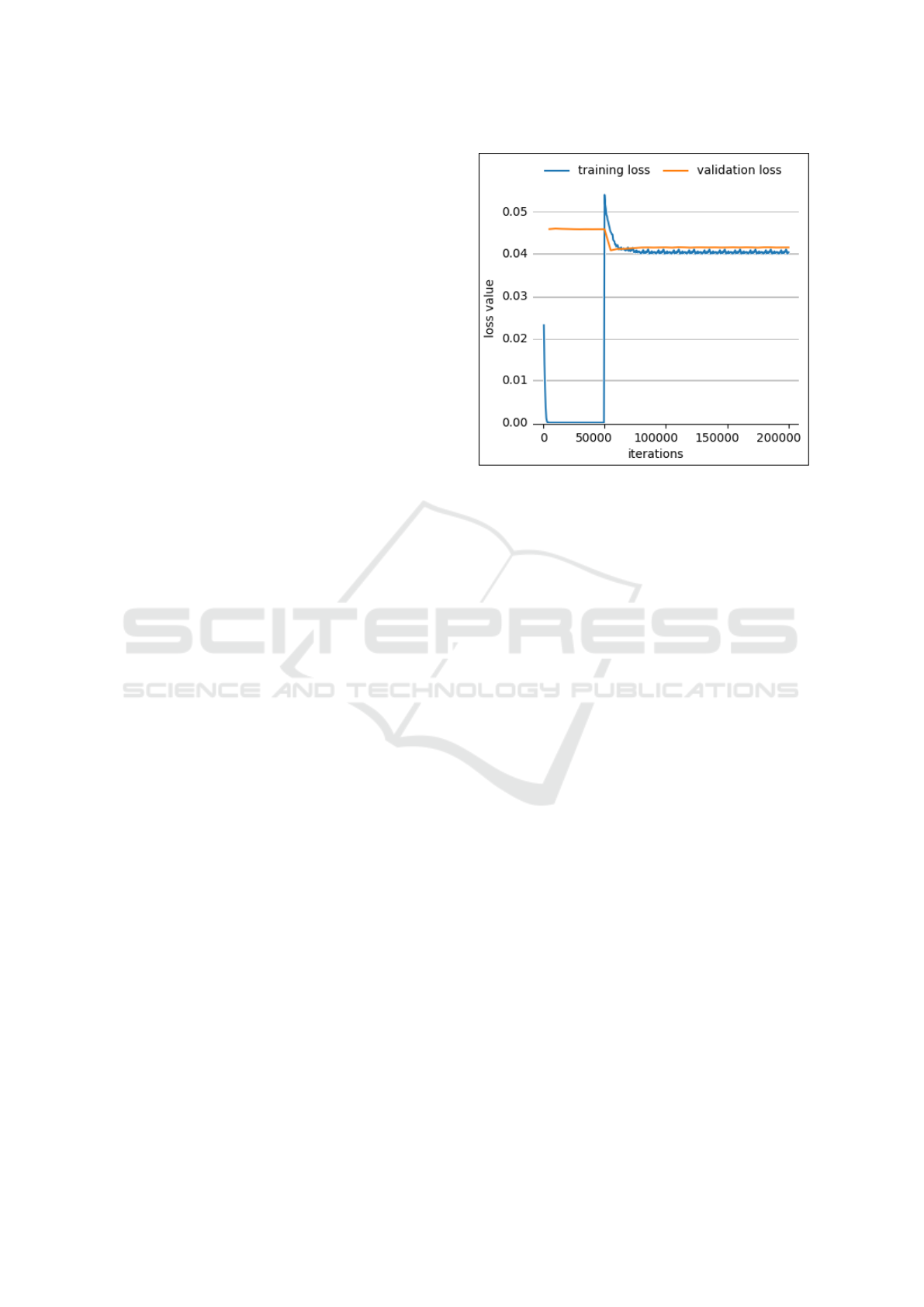
4.2 DPSL Process Evaluation
In this section, the evolution of the loss value throug-
hout a learning process is analysed. The learning pro-
cess has been conducted by the DPSL framework pre-
sented in Section 1. Figure 4 renders the learning
curve for that training process, that is the loss value
for different iteration numbers.
The 100 individuals selected for training (menti-
oned in subsection 4.1) have been coupled with each
other to form a huge number of positive and negative
pairs. This large set of samples has been divided into a
training and a cross-validation set in a 70%-30% pro-
portion.
Although the proposed algorithm has been trained
only using the training set, the loss value, for both the
training and the cross-validation sets, has been repre-
sented, in blue and orange respectively.
The training loss quickly decreases during the first
iterations until it almost achieves the value zero. Ho-
wever, in the iteration 50000 the loss value is drasti-
cally increased. The reason is that 50000, is the value
of the iteration threshold, T
it
, taken by the connection
function, defined by (2). From that iteration, the Ma-
halanobis distance is used as metric distance, dm, to
feed the loss function, (13), instead of the Euclidean
distance, previously used.
Even though the training loss is really low in
the first iterations, that is not the case for the cross-
validation loss. That means the networks have been
over-fitted and the algorithm does not generalises pro-
perly with new samples.
Figure 4: Learning Curve.
Therefore, the model learnt in further iterations,
for instance in the iteration 200,000, has been the one
chosen as definitive to do the experiments, because
both losses values achieve a certain balance at that
point since the validation loss is also reduced from
the iteration T
it
.
This means that the algorithm is able to give a ge-
neralised solution for unknown samples (the test sam-
ples). This fact is due to the proposed Discriminative
Data Structure Analysis, Subsection 3.7, to learn the
Mahalanobis matrix, which codes the view variations
from the two different cameras sets.
4.3 Evaluation Metric
To evaluate the proposed DPSL, a standard re-id
performance measurement has been calculated, the
Cumulative Matching Characteristic (CMC) curve
(Moon and Phillips, 2001).
To obtain the CMC curve, first, every image from
the probe set is coupled with all the images from the
gallery set and the corresponding distance metrics,
dm, are computed. Both sets were defined in Sub-
section 4.1.
Then the CMC curve renders the expectation of
finding the correct match within the top r matches,
for different values of r, called rank. The matches
presenting the lowest values for dm are considered as
the top matches.
4.4 Experimental Results
In order to analyse the effects of using the Mahala-
nobis distance to measure the similarity between two
Deep Parts Similarity Learning for Person Re-Identification
425
person images, we have tested our, Deep Parts Simi-
larity Learning, DPSL, algorithm using both, the Ma-
halanobis and the Euclidean distance as distance me-
trics.
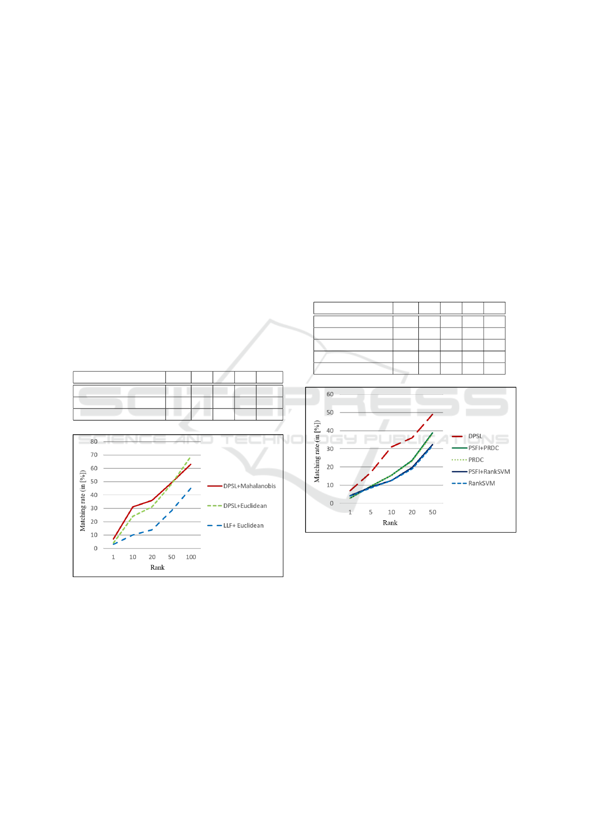
The resulting CMC scores are presented in Table 1
and their corresponding curves are rendered in Figure
5 to make easier a visual comparison.
The scores are generally better for the use of
the Mahalanobis distance, especially in the firsts
ranks which are the most critical ones for the re-
identification task. The reason is that the Mahalanobis
matrix codes the visual camera-to-camera transitions
making the Mahalanobis distance able to cope with
the intra-class variations.
Moreover, with the aim of studying the advanta-
ges of using a deep learning approach to select the
proper features, the Table 1 and Figure 5 also show
the results given by the algorithm presented in (Hirzer
et al., 2012), since this uses low-level features (LLF)
based on colour and texture and they are compared
using also the Euclidean distance as distance metric.
Table 1: CMC scores(in [%]) for different feature extraction
approaches and distances.
Method r=1 10 20 50 100
DPSL+Mahalanobis 7 31 36 49 63
DPSL+Euclidean 4 24 31 48 69
LLF+Euclidean 3 10 14 28 45
Figure 5: CMC curves for different feature extraction ap-
proaches and distances.
The proposed DPSL framework produces better
results because it automatically finds the most salient
features, which causes a remarkable improvement
with respect to the use of low-level hand-crafted fe-
atures.
The main contributions of the proposed DPSL fra-
mework are the deeply learnt weighting, and the dis-
criminative data structure analysis to learn the Maha-
lanobis matrix. For that reason, two methods compa-
risons have been performed with other state-of-the-art
algorithms.
For the first comparison, the following weighting
algorithms have been evaluated and compared with
the proposed DPSL: two Global Feature Importance
(GFI) based methods, the Ranking Support Vector
Machines (Rank-SVM), (Prosser et al., 2010), and
Probabilistic Relative Distance Comparison (PRDC),
(Zheng et al., 2011), and the fusion of both with the
Prototype-Sensitive Feature Importance based met-
hod presented in (Liu et al., 2014).
The obtained CMC scores, for the first ranks, are
listed in Table 2 and the corresponding curves are ren-
dered in Figure 6 to provide a more intuitive compa-
rison representation.
Table 2: Comparison of CMC scores(in [%]) for different
weighting methods.
Method r=1 5 10 20 50
DPSL 7 17 31 36 49
PSFI+PRDC 3 9 16 24 39
PRDC 3 10 15 23 38
PSFI+RankSVM 4 9 13 20 32
RankSVM 4 9 13 19 32
Figure 6: Comparison of CMC curves for different weig-
hting methods.
The proposed DPSL method produces a consi-
derable improvement of the re-identification perfor-
mance, as the CMC scores prove. This is due to the
fact of using a fully connected layer which automa-
tically finds the best weights for each one of the ex-
tracted body part features to combine them forming a
proper person descriptor.
For the second comparison, the Linear Discri-
minant Analysis (LDA) (Fisher, 1936) and Logistic
Discriminant Metric Learning (LDML) (Guillaumin
et al., 2009) algorithms have been tested, which fol-
low a probabilistic approach. The obtained CMC sco-
res are listed in Table 3 and the corresponding curves
VISAPP 2018 - International Conference on Computer Vision Theory and Applications
426
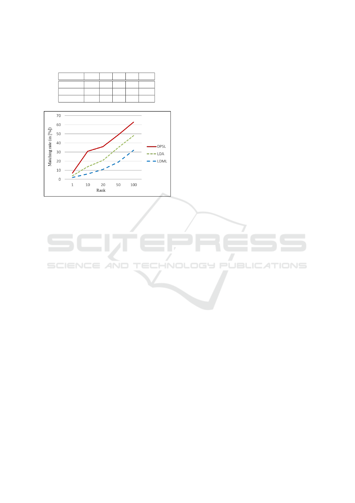
Table 3: Comparison of CMC scores(in [%]) for different
discriminant distance learning methods.
Method r=1 10 20 50 100
DPSL 7 31 36 49 63
LDA 4 14 21 35 48
LDML 2 6 11 19 32
Figure 7: Comparison of CMC curves for different discri-
minant distance learning methods.
are shown in Figure 7.
The CMC scores have been enhanced with the
DPSL method thanks to the adaptive process of
data analysing, conducted in every learning iteration,
which considers the discriminative information given
by the samples labels to create two different features
spaces. One of the features spaces represents the si-
milarity class and the other the dissimilarity class, and
from both, the covariance matrices have been com-
puted and used to code the view-to-view transforma-
tions, related to changes in illumination, resolution,
point of view, etc. All this information is encompas-
sed in the Mahalanobis matrix, reducing the effect of
the intra-class variation and making easier the task re-
identification, whose performance has been remarka-
bly improved by the proposed approach.
5 CONCLUSIONS
The goal of the presented work was to address the per-
son re-identification problem through a Deep Parts Si-
milarity Learning (DPSL) framework, which unifies
the feature and metric selections tasks.
The re-identification of a person in two images be-
comes a important challenge when both representa-
tions are significantly dissimilar, causing intra-class
variations. Some of such variations, like the presen-
ted in resolution, scale, illumination or point of view,
are due to the different location and specifications of
each one of the cameras. Those view-to-view tran-
sitions can be learnt and considered during the re-
identification task to make it easier and improve its
performance.
In this paper, the Mahalanobis matrix has been
proposed to code such information, so the Mahalano-
bis distance has been used to compute the degree of
similarity between a pair of images. The estimation
of that matrix has been conducted with a Discrimi-
native Data Structure Analysis layer, which has been
integrated into the learning framework. In that way
the features and the Mahalanobis matrix learning take
advantage of each other, improving and accelerating
both learning processes simultaneously. This solution
has been compared with other Discriminant Distance
Learning methods, providing successful results.
In addition, the presented unified approach has al-
lowed solving the problem of over-fitting in the fea-
tures learning process, as it has been proved with the
representation of its learning curve.
On the other hand, the variations caused by the
different backgrounds and poses in the images to
compare, have been minimised thanks to a first layer,
which extracts several body parts, independently from
the images scale. This parts extraction layer is based
on a Convolutional Pose Machine (CPM), (Wei et al.,
2016), and it has been integrated into the feature lear-
ning framework, improving the selection of the most
salient features.
The extraction of features for each body part has
been also addressed with the training of deep con-
volutional neural networks, where the use of a fully
connected layer automatically weighs the descriptors
to get the optimal person representation. The evalua-
tion of this approach has resulted in a remarkable im-
provement of the re-identification performance with
respect to other feature selection and weighting met-
hods.
In summary, all these contributions have been uni-
fied in a Deep Part Similarity Learning algorithm,
which follows a Siamese Network architecture. The
proposed approach provides a novel method for me-
asuring the appearance similarity between two per-
son images, which successfully addresses the re-
identification problem, as the experiments have pro-
ved with hopeful and prominent results.
ACKNOWLEDGEMENTS
This work was supported by the Spanish Government
through the CICYT project (TRA2013-48314-C3-1-
R), (TRA2015-63708-R) and Ministerio de Educa-
cin, Cultura y Deporte para la Formacin de Profeso-
rado Universitario (FPU14/02143), and Comunidad
Deep Parts Similarity Learning for Person Re-Identification
427

de Madrid through SEGVAUTO-TRIES (S2013/MIT-
2713).
REFERENCES
Bazzani, L., Cristani, M., and Murino, V. (2013).
Symmetry-driven accumulation of local features for
human characterization and re-identification. Compu-
ter Vision and Image Understanding, 117(2):130–144.
Bazzani, L., Cristani, M., and Murino, V. (2014). Sdalf:
modeling human appearance with symmetry-driven
accumulation of local features. In Person Re-
Identification, pages 43–69. Springer.
Chan-Lang, S., Pham, Q. C., and Achard, C. (2016). Bidi-
rectional sparse representations for multi-shot person
re-identification. In Advanced Video and Signal Ba-
sed Surveillance (AVSS), 2016 13th IEEE Internatio-
nal Conference on, pages 263–270. IEEE.
Cheng, D. S. and Cristani, M. (2014). Person re-
identification by articulated appearance matching. In
Person Re-Identification, pages 139–160. Springer.
Felzenszwalb, P. F. and Huttenlocher, D. P. (2005). Pic-
torial structures for object recognition. International
journal of computer vision, 61(1):55–79.
Fisher, R. A. (1936). The use of multiple measurements in
taxonomic problems. Annals of eugenics, 7(2):179–
188.
G
´
omez-Silva, M. J., Armingol, J. M., and de la Escalera,
A. (2017). Deep part features learning by a normali-
sed double-margin-based contrastive loss function for
person re-identification. In VISIGRAPP (6: VISAPP),
pages 277–285.
Gray, D. and Tao, H. (2008). Viewpoint invariant pede-
strian recognition with an ensemble of localized fea-
tures. Computer Vision–ECCV 2008, pages 262–275.
Guillaumin, M., Verbeek, J., and Schmid, C. (2009). Is that
you? metric learning approaches for face identifica-
tion. In Computer Vision, 2009 IEEE 12th internatio-
nal conference on, pages 498–505. IEEE.
Hirzer, M., Beleznai, C., Roth, P. M., and Bischof, H.
(2011). Person re-identification by descriptive and
discriminative classification. In Scandinavian confe-
rence on Image analysis, pages 91–102. Springer.
Hirzer, M., Roth, P., K
¨
ostinger, M., and Bischof, H.
(2012). Relaxed pairwise learned metric for person
re-identification. Computer Vision–ECCV 2012, pa-
ges 780–793.
Jia, Y., Shelhamer, E., Donahue, J., Karayev, S., Long, J.,
Girshick, R., Guadarrama, S., and Darrell, T. (2014).
Caffe: Convolutional architecture for fast feature em-
bedding. In Proceedings of the 22nd ACM internatio-
nal conference on Multimedia, pages 675–678. ACM.
Khan, F. M. and Br
´
emond, F. (2016). Unsupervised data
association for metric learning in the context of multi-
shot person re-identification. In Advanced Video and
Signal Based Surveillance (AVSS), 2016 13th IEEE In-
ternational Conference on, pages 256–262. IEEE.
Koestinger, M., Hirzer, M., Wohlhart, P., Roth, P. M., and
Bischof, H. (2012). Large scale metric learning from
equivalence constraints. In Computer Vision and Pat-
tern Recognition (CVPR), 2012 IEEE Conference on,
pages 2288–2295. IEEE.
Layne, R., Hospedales, T. M., and Gong, S. (2014).
Attributes-based re-identification. In Person Re-
Identification, pages 93–117. Springer.
Liu, C., Gong, S., Loy, C. C., and Lin, X. (2014). Evaluating
feature importance for re-identification. In Person Re-
Identification, pages 203–228. Springer.
Ma, B., Su, Y., and Jurie, F. (2014). Discriminative image
descriptors for person re-identification. In Person Re-
Identification, pages 23–42. Springer.
Moon, H. and Phillips, P. J. (2001). Computational and
performance aspects of pca-based face-recognition al-
gorithms. Perception, 30(3):303–321.
Munaro, M., Fossati, A., Basso, A., Menegatti, E.,
and Van Gool, L. (2014). One-shot person re-
identification with a consumer depth camera. In Per-
son Re-Identification, pages 161–181. Springer.
Oreifej, O., Mehran, R., and Shah, M. (2010). Human iden-
tity recognition in aerial images. In Computer Vision
and Pattern Recognition (CVPR), 2010 IEEE Confe-
rence on, pages 709–716. IEEE.
Prosser, B., Zheng, W.-S., Gong, S., Xiang, T., and Mary,
Q. (2010). Person re-identification by support vector
ranking. In BMVC, volume 2, page 6.
Roth, P. M., Hirzer, M., K
¨
ostinger, M., Beleznai, C., and
Bischof, H. (2014). Mahalanobis distance learning for
person re-identification. In Person Re-Identification,
pages 247–267. Springer.
Rumelhart, D. E., Hinton, G. E., and Williams, R. J. (1988).
Learning representations by back-propagating errors.
Cognitive modeling, 5(3):1.
S
´
anchez, J., Perronnin, F., Mensink, T., and Verbeek, J.
(2013). Image classification with the fisher vector:
Theory and practice. International journal of com-
puter vision, 105(3):222–245.
Wei, S.-E., Ramakrishna, V., Kanade, T., and Sheikh, Y.
(2016). Convolutional pose machines. In Proceedings
of the IEEE Conference on Computer Vision and Pat-
tern Recognition, pages 4724–4732.
Yi, D., Lei, Z., Liao, S., and Li, S. Z. (2014). Deep me-
tric learning for person re-identification. In Pattern
Recognition (ICPR), 2014 22nd International Confe-
rence on, pages 34–39. IEEE.
Zhang, Y. and Li, S. (2011). Gabor-lbp based region covari-
ance descriptor for person re-identification. In Image
and Graphics (ICIG), 2011 Sixth International Confe-
rence on, pages 368–371. IEEE.
Zheng, W.-S., Gong, S., and Xiang, T. (2011). Person re-
identification by probabilistic relative distance com-
parison. In Computer vision and pattern recognition
(CVPR), 2011 IEEE conference on, pages 649–656.
IEEE.
VISAPP 2018 - International Conference on Computer Vision Theory and Applications
428
