
Mathematical Programs and Computations for a Class of
Anti-aircraft Mission Planning Problems
Trang T. Nguyen, Trung Q. Bui, Bang Q. Nguyen and Su T. Le
C4I Department, Viettel Research and Development Institute, Vietnam
Keywords:
Military, Theater Defense Distribution, Mixed Integer Programming.
Abstract:
The theater defense distribution is an important problem in the military that determines strategies against a
sequence of offensive attacks in order to protect his targets. This study focuses on developing mathematical
models for three important defense problems that generate anti-aircraft mission plans for a group of missile
battalions. The simple Anti-aircraft Launching Assignment problem specifies number of missiles should be
launched from each battalion to each fleet of attacking aircraft to maximize the defensive effectiveness, pro-
vided that the locations of missile battalions are given. On the other hand, the Anti-aircraft Mission Planning
problem maximizes the defender’s effectiveness using all his available battalions, while the Inverse Anti-
aircraft Mission Planning problem computes necessary weapon resources (battalions and their missiles) to
obtain a given defensive effectiveness value. The proposed formulations are Integer Programs and proved as
NP-hard. A comprehensive set of experiments is then evaluated to show that these proposed programs can be
applied to solve fast real-life instances to optimality.
1 INTRODUCTION
The Theater Distribution Model (TDM) is specifi-
cally designed to support the combatant commander
to ensure his effective plans within area of operations
(Shalikashvili, 1996). Most of researches in the litera-
ture focus on the military theater distribution problem
associated with determining positions of defender’s
missile battalions within a potentially geographical
region (Shalikashvili, 1993). In most cases, the de-
fender faces with so many risks from terrorist attacks
of all kinds. The work we research here is directly
motivated by such one risk assessment: surface-to-
air missile battalions defense against many fleets of
penetrating aircraft. Beside the role of specializing
anti-aircraft, missile battalions in an air defense sy-
stem also protect a target such as capital, political
area, economy or military center. The Department
of Air Defense and Air Force has conducted some
risk assessment exercises and estimated risks of many
attack possibilities. One area that is still undeve-
loped is an algorithm for determining an intelligent
package of missile battalion’s actions to aircraft at-
tack. A missile battalion package consisting of only
one missile type might be ineffective but when se-
veral types of missiles are combined properly, they
confidently destroy the attacking aircraft and protect
their target. More precisely, we develop mathemati-
cal formulations for anti-aircraft mission planning ef-
fectively for a group of missile battalions. A missile
battalion is considered as a fundamental tactical buil-
ding block which recruits or conscripts in one geo-
graphical area assigned by a feudal lord. Given some
threat, the defender must decide where to locate de-
fensive missile battalions among potential locations
and how they should engage fleets of attacking air-
craft. We express the defender’s courses of action as
following mathematical optimization problems. The
first and simple problem is the Anti-aircraft Laun-
ching Assignment (ALA) that computes number of
missiles should be launched from each battalion to
each fleet of attacking aircraft to maximize the de-
fensive effectiveness, provided that the locations of
missile battalions is given. On the other hand, the
Anti-aircraft Mission Planning problem (AMP) cal-
culates not only the launching assignment for the bat-
talions but also locations of the battalions while In-
verse Anti-aircraft Mission Planning problem (IAMP)
computes necessary weapon resources, battalions’ lo-
cations, and a launching assignment to obtain a gi-
ven effectiveness threshold. The most valuable con-
tribution of this paper comes from the statements and
practical mathematical formulations for these three
crucial problems in the TDM class. The ALA arises
Nguyen, T., Bui, T., Nguyen, B. and Le, S.
Mathematical Programs and Computations for a Class of Anti-aircraft Mission Planning Problems.
DOI: 10.5220/0006539801550163
In Proceedings of the 7th International Conference on Operations Research and Enterprise Systems (ICORES 2018), pages 155-163
ISBN: 978-989-758-285-1
Copyright © 2018 by SCITEPRESS – Science and Technology Publications, Lda. All rights reser ved
155

in the crowded cities where there are not many choi-
ces for locating missile battalions while the AMP is
necessarily tackled in sparsely populated area. On the
contrary, the IAMP is necessarily considered when
the protected target should not be fallen in any ca-
ses. Although these problems are proven as NP-hard,
the computational results show the efficient of our for-
mulations since they can be applied directly to solve
fast real-life instances to optimality. The message
is that, with the validation of experienced soldiers,
we have gained confidence that the formulations have
significant implementation in any defender’s combat
field. The rest of paper is organized as follows. In
Section 2, we state the problems, formulate them as
mixed integer programs as well as prove their hard-
ness. The experimental results are reported and ana-
lyzed in Section 3. Finally, we conclude the paper and
draw some future directions in Section 4.
The TDM has been motivated and validated for
both defensive side and offensive side in general
((Robert, 2006), (Crino and Moore, 2004), (Jackson,
1989), (Studies and Agency, 1992), (Brian, 1994),
(Seichter, 2005), (Moore, 2002), (Brown et al., 2008)
). Some of these studies have been developed into
mathematical models which are related to the AMP
can be classified as the Weapon-Target Assignment
(WTA)and the Defender- Attacker Model (DAM).
The WTA is the assignment of weapon to the hos-
tile target in order to protect assets, which can be
formulated as a nonlinear integer programming pro-
blem and is known to be NP-hard complete. Although
several heuristic methods have been propose for sol-
ving the WTA, such as genetic algorithm, tabu search,
simulated annealing, and variable neighborhood se-
arch ((Murphey, ), (Tokgoz and Bulkan, 2013)), an
integer programming and network flow-based lower
bounding method has been introduced in (Ahuja Ra-
vindra and James, 2007). An instance of DAM in a
fast theater model is introduced in (Seichter, 2005),
which is built upon the existing air model. The air
strike attacker’s main objective is maximizing target
value destroyed by killing as many targets with high
values as possible, while the ground combat wants
to minimize its own losses. The resulting model is
a Mixed Integer Program (MIP) finding an optimal,
actively defensive actions by the ground force that
can significantly reduce the air attacker’s effective-
ness. The defender-attacker problem is continued stu-
dying in (Moore, 2002), in which a new methodo-
logy for strategy optimization under uncertainty has
been proposed. The authors describe the implemen-
tation of a genetic programming algorithm to deter-
mine an optimized evasion strategy for the extended
two-dimensional pursuer-evader problem under con-
ditions of uncertainty about the type of pursuer. The
DAM model is also applied to defender’s risk asses-
sment and mitigation,(Brown et al., 2008).
2 PROBLEM FORMULATIONS
We now state and formulate the anti-aircraft mission
planning problems. The complexity of these pro-
blems is also discussed at the end of this section.
2.1 Problem Descriptions
Direction
Height (km)
π
4
π
2
3π
4
π
5π
4
3π
2
7π
4
2π
1
2
4
6
8
10
22
Oppressive fleet: F15, F16, F14
Bomb fleet: F15, F16
Diversionary fleet
Escort fighter fleet
Bomb fleet: B52, B1, B2
Radar-jamming fleet: EF111A, EC130H, EA6B
Reconnaissance fleet: TR1, U2, SR71
Figure 1: An example of an attacking plan.
Suppose that the attacker’s plan can be observed
by an intelligence system of the defender and is des-
cribed as follows. In the offensive side, the attacker
strikes the target by a group of fleets of attacking ai-
rcraft. For a sake simplicity, from now on, the term
“fleet” is used stead of “fleet of attacking aircraft”.
Each fleet is organized by a group of aircraft which
have same missions such as carrying bombs or ma-
king radar noise; enter the theater at same height, di-
rection; and fly with same velocity. Each fleet is asso-
ciated with a weight of importance depending mainly
on its mission. Figure 1 illustrates an attacking plan,
in which the horizontal axis represents the directions
of the fleets, considered as angles between attacking
directions and a predefined axis; while the vertical
axis represents the height of the fleets. There are se-
ven fleets at different heights, directions and veloci-
ties, drawn by seven arrows. The color of the arrows
reflects the fleets’ weights. For instance, the darkest
arrow describes the fleet with the highest weight, car-
rying bombs such as B52, B1, B2. Further, flying po-
sitions of aircraft in a fleet must be captured in detail,
for example, a flying position of a four-aircraft fleet is
illustrated in Figure 2.
In the defensive side, the defender’s responsibility
is engaging fleets to protect its point target. In or-
ICORES 2018 - 7th International Conference on Operations Research and Enterprise Systems
156
2.5km 5km 2.5km 5km 2.5km 10km 3km
Figure 2: An example of an attacking fleet.
der to formulate a class of anti-aircraft mission plan-
ning problems, we take into account following fac-
tors. The first one is critical radius corresponding to
each fleet that defines a critical circle centered at the
target. The defender has to make a defensive plan
such that no attacking aircraft in that fleet is able to
get inside that circle. This critical radius is compu-
ted depending on the height, velocity of that fleet and
type of bombs carried by that fleet. For instance, in
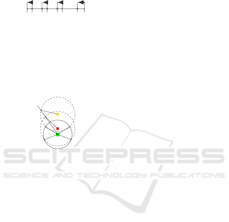
Figure 3, the point target is described by the green
rectangle with critical radius OX corresponding to a
fleet coming from the AO direction. The second fac-
A
O
B
C
D
B
1
B
2
X Y
V W
Figure 3: An example of influence of battalion’s locations
on their firepower capabilities.
tor is action range of a battalion corresponding to a
fleet that can be understood as a fleet’s flying path
where the fleet will be intercepted by that battalion.
In Figure 3, the action range of battalion B
1
is CD
segment, where D is the intersection of the attacking
direction AO and the critical circle, and C is the inter-
section of the direction AO and the circle centered at
B
1
of radius B
1
C which is defined as the long range
of missiles belonging to that battalion. Similarly, the
action range of battalion B
2
is BD segment. The third
factor maximum launches representing firepower ca-
pabilities of a battalion can be seen as maximum num-
ber of missiles that can be launched from the battalion
to the fleet in its action range. This number is calcula-
ted basing on the type of missile, number of missiles
in that battalion, as well as the shortest time between
two successive launches. The fourth factor is the ex-
pected number of killed aircraft of a fleet caused by a
battalion in a number of launches. This value can be
estimated by number of missiles, probability of kill,
defensive mode related to each fleet, and set of coeffi-
cients corresponding to each missile battalion such as
technical coefficient, control coefficient, and complex
coefficient of combat. Lastly, a minimum distance be-
tween each pair of battalions is required to avoid ra-
dar jamming between missiles in the battalions. Note
that if two battalions locate at a same position, this
constraint can be ignored. As a defender, we would
like to measure the result of our defense. An effective
criterion is then introduced as defensive effectiveness,
calculated by fraction between value of killed aircraft
and value of all aircraft in attacking fleets. The effecti-
veness is strongly influenced by battalions’ locations,
that motivates us to study an adaptable, efficient, and
cost-effective process to analyse missile battalion de-
fense against aircraft threats. Three problems propo-
sed in this paper, the ALA, AMP and IAMP, belong
to the defensive side, where the defender preserves a
point target. The attacker’s plan including all infor-
mation about the offensive side stated above is sup-
posed to be observed clearly by the intelligence sy-
stem of the defender. While in the AMP, the defender
not only finds optimal locations for missile battalions
but also indicates numbers of missiles launched from
battalions to fleets; in the ALA, the defenders is not
required to find locations for battalions. We consi-
der now somewhat inverse version of the AMP, the
IAMP. Assume, in particular, that the defender has
a set of battalions, in stead of using all battalions to
maximize his defensive effectiveness, one generates
a defensive mission plan such that the corresponding
effectiveness is greater than or equal to a given value.
The detailed mathematical programs of these models
are proposed in Section 2.2.
2.2 Mathematical Programs
For a simplicity of presentation, we first introduce
some indices and notations.
Inputs
• B: set of missile battalions;
• F: set of fleets of attacking aircraft;
• L: set of potential locations for battalions;
• For a battalion b ∈ B, denote m(b) and c(b) by
number of missiles distributed to b and cost of a
missile of b, respectively;
• For a fleet f ∈ F, denote n( f ) and w( f ) by num-
ber of aircraft in fleet f and weight of that fleet,
respectively;
• For a pair (b, f ) (b ∈ B, f ∈ F), denote t(b, f ) by
the maximum number of missiles that battalion b
is able to launch to fleet f in its action range;
• Last, for a triple (b, f ,t) (b ∈ B, f ∈ F and t ∈ Z
+
),
denote e(b, f ,t) by the expected number of killed
aircraft in fleet f caused by t missiles launched
from battalion b to fleet f .
Mathematical Programs and Computations for a Class of Anti-aircraft Mission Planning Problems
157

2.2.1 ALA Mathematical Program
Given the locations of battalions, the objective of the
ALA is to compute number of missiles should be
launched from each battalion toward each fleet such
that the defensive effectiveness is maximized. This
program arises naturally in real-life instance when the
target and battalions are firmly positioned in a given
area. To formulate the ALA program, we introduces
binary variables x
b, f ,t
where b ∈ B, f ∈ F and t ∈ Z
+
indicating that whether t missiles are launched from
battalion b to fleet f or not. The mathematical pro-
gram of the ALA problem can be stated as a mixed
integer program as follows.
Max
∑
f ∈F
w( f )
∑
b∈B
t(b, f )
∑
t=1
e(b, f ,t)x
b, f ,t
n( f )
(1a)
s.t.
∑
f ∈F
t(b, f )
∑
t=1
tx
b, f ,t
≤ m(b), ∀b ∈ B
(1b)
∑
b∈B
t(b, f )
∑
t=1
e(b, f ,t)x
b, f ,t
≤ n( f ), ∀ f ∈ F
(1c)
x
b, f ,t
∈ {0,1}, ∀b ∈ B, f ∈ F,t ∈ {1,.. .,t(b, f )}.
(1d)
In this program, the objective function (1a) is the
defensive effectiveness which can be calculated as the
fraction between the value of killed aircraft and the
value of aircraft in these fleets. Constraints (1b) sim-
ply stipulate that the number of launched missiles of
each battalion should not be greater than its given
load-out. Constraints (1c) ensure the number of ai-
rcraft destroyed in a fleet do not exceed the number
of aircraft in that fleet; while the launching times con-
straints are hidden in (1b) and (1c) since t takes values
in [1,t(b, f )]. The variables are restricted to be binary
in constraints (1d).
2.2.2 AMP Mathematical Program
We consider now a situation that the defender need to
decide where to locate missile battalions among a set
of limited number of available locations and missiles
to distribute a defensive mission plan that maximizes
his defensive effectiveness. The AMP can be viewed
as an extension of the ALA model. The AMP formu-
lation introduces more variables representing locati-
ons of battalions and missile-distance constraints de-
fining lower bounds for geographic distances between
battalions at different locations. In addition to notati-
ons, variables and constraints introduced in the ALA
formulation, the AMP considers more categories of
factors as follows.
Inputs:
• For a pair of locations (l
i
,l
j
) (l
i
,l
j
∈ L), denote
d(l
i
,l
j
) by the geometric distance between l
i
and
l
j
;
• For a pair of battalions (b
i
,b
j
) (b
i
,b
j
∈ B), denote
d(b
i
,b
j
) by the minimum distance between b
i
and
b
j
if they are located at two different positions;
• For each triple (b,l, f ) (b ∈ B,l ∈ L, f ∈ F), de-
note t(b,l, f ) by the maximum number of missi-
les that battalion b located at l is able to launch to
fleet f in its action range;
• For a quadruple (b,l, f ,t) (b ∈ B, l ∈ L, f ∈ F and
t ∈ Z
+
), e(b,l, f ,t) indicates the expected number
of killed aircraft in fleet f caused by t missiles
launched from battalion b located at l to fleet f .
Further, we introduce binary variables y
b,l
where
b ∈ B,l ∈ L, indicating whether battalion b locates
at location l or not. Second, binary variables z
b,l, f ,t
where b ∈ B,l ∈ L, f ∈ F and t ∈ Z
+
, state that if t
missiles are launched from battalion b located at lo-
cation l to fleet f . In addition to constraints given
in the ALA formulation, the AMP requires minimum
distance between any two battalions such that if batta-
lions b
i
and b
j
locate at location l
i
and l
j
respectively,
then
d(l
i
,l
j
) ≥ d(b
i
,b
j
), ∀b
i
6= b
j
,l
i
6= l
j
(2)
The MIP model for the AMP problem can be repre-
sented as:
Max
∑
f ∈F
w( f )
∑
l∈L
∑
b∈B
t(b,l, f )
∑
t=1
e(b,l, f ,t)z
b,l, f ,t
n( f )
(3a)
s.t.
∑
l∈L
y
b,l
= 1, ∀b ∈ B
(3b)
∑
l∈L
∑
f ∈F
t(b,l, f )
∑
t=1
tz
b,l, f ,t
≤ m(b),∀b ∈ B
(3c)
(2 − y
b
i
,l
i
− y
b
j
,l
j
)∞ + y
b
i
,l
i
d(l
i
,l
j
) ≥ d(b
i
,b
j
)
∀b
i
,b
j
∈ B,b
i
6= b
j
,∀l
i
,l
j
∈ L,l
i
6= l
j
(3d)
∑
l∈L
∑
b∈B
t(b,l, f )
∑
t=1
e(b,l, f ,t)z
b,l, f ,t
≤ n( f ),∀ f ∈ F
(3e)
∑
f ∈F
t(b,l, f )
∑
t=1
z
b,l, f ,t
≤ y
b,l
,∀b ∈ B, l ∈ L
(3f)
y
b,l
;z
b,l, f ,t
∈ {0,1}, ∀b ∈ B,l ∈ L, f ∈ F,
t ∈ {1,. . .,t(b,l, f )}.
(3g)
ICORES 2018 - 7th International Conference on Operations Research and Enterprise Systems
158

In the AMP formulation, the defender’s objective
is maximizing its effectiveness (3a) which is the sum
of fractions of expected number of killed aircraft and
number of aircraft n( f ) for all fleets while considering
additionally the importance weights of these fleets.
Constraints (3b) simply limit each missile battalion
to one location. Constraints (3c) stipulate that the
number of launches from each battalion should not
be greater than its given number of missiles. Con-
straints (3d) describes the missile-distance constraints
(2), showing that if two missile battalions b
i
and b
j
are at locations l
i
and l
j
where l
i
6= l
j
, respectively,
the distance between these battalions must be grea-
ter than a required minimum distance
¯
d(b
i
,b
j
). Con-
straints (3e) define upper bounds for number of air-
craft in these fleets. Constraints (3f) tell us that there
are some missiles launched from a location to a fleet
if and only if there exists at least one missile batta-
lion located at that location. Lastly, constraints (3g)
indicate that x
b,l
,y
b,l, f ,t
where b ∈ B,l ∈ L, f ∈ F,t ∈
{1,... ,t(b,l, f )} are binary variables.
2.2.3 IAMP Mathematical Program
An other significant situation that usually appears in
the real combat field is the inverse AMP problem, the
IAMP. Assume, in particular, that the defender has
a set of battalions, in stead of using all battalions to
maximize his defensive effectiveness, one generates
a defensive mission plan such that the corresponding
effectiveness is greater than or equal to a given value
with the lowest cost. Intuitively, one would like to lo-
cate defensive battalions as well as compute number
of missiles with the lowest cost such that its effective-
ness is at least γ (such as γ = 0.5, 0.6,...). In addition
to the inputs introduced in the ALP and the AMP, the
IAMP program need some more notations.
Inputs:
• For a battalion b ∈ B, denote c(b) by the cost of a
missile of b;
• For each pair (b, l) of a battalion b ∈ B and a lo-
cation l ∈ L, c(b,l) refers to the cost of allocating
battalion b at location l;
Further, the IAMP mathematical formulation in-
troduces more integer variables u
b
∈ Z
+
, indicating
number of missiles launched from battalion b ∈ B.
The mathematical program for the IAMP is given as:
The objective of this formulation is to minimize
the total cost (4a) that is calculated by sum of esta-
blishing battalion cost and launched missile cost on
these battalions. Constraints (4b) are different from
(3b) since not every missile battalion is required to
locate at some location. Constraint (4d) requires the
obtained effectiveness be at least a given value, γ. The
number of missiles on each battalion is set at con-
straints (4e) while its upper bound has been given
in constraints (4f). The other constraints are similar
to ones in the AMP formulation given in constraints
(4c), except that number of launched missiles are in-
teger variables as in constraints (4g).
Min
∑
b∈B
∑
l∈L
c(b,l)y
b,l
+
∑
b∈B
c(b)u
b
(4a)
s.t.
∑
l∈L
y
b,l
≤ 1, ∀b ∈ B
(4b)
Constraints(3c),(3d),(3e),(3 f ), (3g)
(4c)
∑
f ∈F
w( f )
∑
l∈L
∑
b∈B
t(b,l, f )
∑
t=1
e(b,l, f ,t)z
b,l, f ,t
n( f )
≥ γ,
(4d)
u
b
−
∑
l∈L
∑
f ∈F
t(b,l, f )
∑
t=1
tz
b,l, f ,t
= 0, ∀b ∈ B
(4e)
u
b
≤ m(b)
∑
l∈L
y
b,l
, ∀b ∈ B
(4f)
u
b
∈ Z
+
, ∀b ∈ B
(4g)
where γ ∈ [0, 1] is a given effectiveness value.
Note here that, the ALA and the AMP always re-
sult in an optimal solution with the effectiveness be-
longing to [0, 1], while the IAMP sometimes returns to
no solution in case the weapon resources are not suf-
ficiently available to reach the expected effectiveness.
Further, one of the difficulties to deal with these pro-
grams is to define the values of parameters that suppo-
sed to be known. This study clarifies how to compute
the expected number of killed aircraft, the maximum
number of launches and the minimum distance bet-
ween two missiles for special situation of a defensive
missile battalion plan against aircraft attack, that can
be found in the Appendix.
2.3 NP-Hardness
The NP-completeness is indicated as the complexity
of these mathematical programs in this section.
Theorem 1. The ALA is NP-complete.
Proof. To prove this, we reduce the 3-Partition Pro-
blem (3PP) to the decision problem of ALA since the
3PP is known as NP-complete (Garey and Johnson,
1990).
Recall that in the 3PP, we are given a multi-set S
of 3b positive integers i
1
,i
2
,... , i
3b
, where the value
of every element in the set belongs to interval (
C
4
,
C
2
),
for a positive integer C; and we are asked to decide if
Mathematical Programs and Computations for a Class of Anti-aircraft Mission Planning Problems
159

there are b disjoint subsets of S such that sum of all
elements in each subset equals to C.
For any instance of the 3PP, an instance of the de-
cision problem of ALA is simultaneously created as
follows: The set of battalion B is initialized by b mis-
sile battalions; each battalion is allocated 3 missiles;
the set of fleets includes 3b fleets, f
1
, f
2
,... , f
3b
(each
positive integer in the 3PP instance corresponds to a
fleet in the instance of the decision problem of ALA);
each fleet is formed by just one aircraft; each batta-
lion can launch at most one missile to each fleet; the
expected number of killed aircraft is
i
k
C
(
i
k
C
∈ (
1
4
,
1
2
) )
when one missile is launched from any battalion to a
fleet f
k
; for all k ∈ [1, 2, ...,3b], and the lower bound
on the defensive effectiveness is set to 1.
As a result, the 3PP instance has a partition into
b disjoint subsets, sum of elements in each subset
is equal to C, if and only if all battalions located at
the unique location, each battalion launches exactly 3
missiles to 3 fleets and the defender’s effectiveness re-
aches to its ideal value of 1 or all fleets are destroyed
completely. Thus 3PP reduces to the question whet-
her the decision problem of the ALA has a solution
or not. Thus, a pseudo polynomial reduction has been
given, showing that the ALA is NP-complete.
The NP-completeness of the AMP and the IAMP
are proved in the same way as above.
3 EXPERIMENTS
This section dedicates to report and analyze experi-
mental results on variety of instances for the ALA,
AMP and IAMP. For each problem, we generated
randomly 15 instances with the help of experienced
soldiers to make them real and reliable. The coef-
ficients used to generate instances were carefully ex-
tracted from the historical data and technical guides of
missiles S-75 and S-125. The mathematical formula-
tions for the ALA, AMP and IAMP were implemen-
ted in C++ programming language, using IBM Ilog
Cplex Concert Technology, version 12.5. The stan-
dard cuts of Cplex were automatically added. Since
the number of constraints (3d) in the AMP and IAMP
programs is large and they belong to Miller-Tucker-
Zemlin class (Miller et al., 1960), these constraints
are treated as lazy constraints to reduce the computa-
tion time as follows. At the beginning of resolution,
these constraints are all relaxed. Each time, an inte-
ger feasible solution is counted at a node in the search
tree, this solution is checked for the satisfiability of all
these constraints, all violated constraints are injected
more in the model. This cut-addition strategy always
Table 1: Experimental results for the ALA.
Instances Branch-and-Cut
No. b f Gap Eff. Time
1 5 5 0 0.246 0.004
2 7 8 0 0.462 0.005
3 6 5 0 0.742 0.012
4 6 8 0 0.546 0.025
5 7 5 0 0.673 0.004
6 10 10 0.02 0.767 7202.291
7 10 10 0 0.706 21.608
8 10 10 0 0.648 0.083
9 10 10 0.04 0.815 7201.130
10 10 10 0 0.787 2.292
11 10 10 0 0.780 142.796
12 10 10 0.02 0.699 7200.970
13 10 10 0 0.521 1.129
14 10 10 0 0.776 0.252
15 10 10 0 0.999 0.024
ensures the returning solution is correct since all con-
straints (3d) are strictly respected. All computations
were performed in multi-thread mode on a compu-
ter with an Intel Core i7-479 CPU, 3.6 GHz, and 4
GB RAM running Ubuntu version 16.4, 64 bits. A
time limit of 2 hours of CPU time was set for each
instance resolution. All computational results for the
ALA, AMP and IAMP are respectively indicated in
Table 1, 2 and Table 3. The columns in the tables
have the following meanings: No.: Instance number,
b: Number of battalions, m: Number of missiles in
each battalion, l: Number of potential locations, f :
Number of attacking aircraft fleets, Gap: Gap (%) be-
tween the optimal solution of the integral relaxation
of an integer program and integer feasible solution of
that program found so far, Eff.: Defensive effective-
ness value, and Time: Overall CPU time in seconds.
Considering the first five instances in Table 1
where the number of battalions and the number of
fleets are small as the size of a regiment, the Cplex
solver gives optimal solutions very fast. In the instan-
ces (6,9,12), it takes the Cplex solver about 2 hours to
get its best solution, but not the optimal solution. On
the other aspect, it can be seen from instance 8 that the
optimal solution is easily achieved by the Cplex sol-
ver in lest than 1 second. It may be concluded from
the numerical results that the Cplex solver runs fast
and achieves optimal solutions in small size instances
but sometimes it takes several hours to obtain its best
solution.
In reality, the practical AMP usually allocates a
missile regiment of 4 to 6 missile battalions to pro-
tect an important target which is attacked by 5 to 8
attacking aircraft fleets. Instances of those sizes can
be solved so fast by our formulation as report in the
ICORES 2018 - 7th International Conference on Operations Research and Enterprise Systems
160

Table 2: Experimental results for the AMP.
Instances Branch-and-Cut
No. b l f Gap Eff. Time
1 7 38 8 0 0.717 0.63
2 6 8 5 0 0.922 508.87
3 5 58 8 0 0.619 1.52
4 7 50 5 0 1.000 0.50
5 5 83 8 0 0.488 0.65
6 10 100 10 0 1.000 7.67
7 10 100 10 0 0.701 212.89
8 10 100 10 0 0.7919 5.11
9 10 100 10 0 0.7819 172.56
10 10 100 10 0 0.8143 9.66
11 10 100 10 0 0.633 49.81
12 10 100 10 0.02 0.913 7201.38
13 10 100 10 0.05 0.936 7211.39
14 10 100 10 0.07 0.91089 7217.53
15 10 100 10 0.01 0.7099 7201.81
first five rows of Table 2, specially instances (1, 4,5)
of these sizes were solved in less than one second.
This result motivates us to increase the size of test in-
stances up to 10 battalions, 100 locations and 10 fleets
to evaluate the tackling ability of the formulation. In
the time limit of 2 hours, the 11 easy instances (obtai-
ned optimal solutions by Cplex solver) among 15 in-
stances were completely solved to optimality, most of
them take less than 1 minutes; while the 4 hard instan-
ces (not obtained optimal solutions by Cplex solver)
were solved nearly to optimality since the gaps are
so small (0.01% − −0.07%). Although 10 last test
instances have same sizes in term of the number of
battalions, the number of fleets and the number of lo-
cations, the computational difficulty is different. This
diversification comes from the geographic of the po-
tential locations. In comparison to defensive effecti-
veness of easy instances, the hard ones have greater
effectiveness. Sets of available missile battalions in
IAMP instances were generated around 20 battalions
that are larger than the ones used in Table 2. Among
15 instances in Table 3, there are 9 easy instances
solved to optimality in less than 30 seconds, while
5 hard instances were not completely solved in the
time limit, and one instance (No. 15) returned to “Out
of memory” error during the resolution. Similar to
hard AMP instances, the hard IAMP instances gene-
rate very large search trees that may cause no feasi-
ble solution. It is essentially seen that the easy IAMP
instances correspond to reasonable effectiveness va-
lues, while the hard IAMP instances usually are as-
sociated with high effectiveness values. These expe-
rimental results were validated and recommended by
the experienced soldiers that this formulation should
be packaged for the purpose of training and integrated
into a C4I system.
Table 3: Experimental results for IAMP.
Instances Branch-and-Cut
No. b m l f Eff. Gap Time
1 21 12 56 11 0.72 0 18.6
2 21 12 41 11 0.81 0 5.6
3 22 12 42 12 0.97 0.83 7209.9
4 20 12 45 10 0.52 0 11.7
5 21 12 51 11 0.57 0 20.5
6 24 12 54 14 0.98 0.05 7213.7
6 23 12 48 13 0.46 0 9.8
8 23 12 58 13 0.91 0.12 7210.6
9 22 12 47 12 0.71 0 22.1
10 21 12 41 11 0.56 0 29.8
11 23 12 48 13 0.94 0.12 7225.7
12 20 12 55 10 0.84 0.09 7217.6
13 22 12 47 12 0.44 0 8.6
14 22 12 47 12 0.65 0 15.2
15 22 12 57 12 0.60 Out of memory
4 CONCLUSION
In this paper, we formulated three problems in the
class of defensive missile battalions mission planning
against aircraft attack model, that support defensive
decision makers not only decide where to locate their
missile battalions, but also point out that how many
missiles should be launched from each battalion to
each attacking aircraft fleet. The mathematical for-
mulations are IPs, proved as NP-hard. These mathe-
matical programs were implemented and experimen-
ted on test instances generated basing on the help of
experienced veterans, in which parameters on proba-
bility of kill, maximum number of launches, as well
as minimum distance between two battalions, were
pre-processed for a particular set of defensive battali-
ons and aircraft attack. The numerical results provide
the incidence that the proposed formulations should
be widely applied in real-life combat field. As future
works, we intend to formulate and tackle other vari-
ance of the defensive distribution models.
REFERENCES
Ahuja Ravindra, Kumar Arvind, J. K. and James, O. (2007).
Exact and heuristic algorithms for the weapon-target
assignment problem. Operations Research, 55(6).
Brian, J. (1994). An air mission planning algorithm for a
theater level combat model. Master thesis, Air force
Institute of Technology.
Brown, G., Carlyle, M., and Wood, K. (2008). Applying
defender-attacker optimization to terror risk asses-
sment and mitigation. Calhoun, the NPS Institutional
Archive.
Mathematical Programs and Computations for a Class of Anti-aircraft Mission Planning Problems
161

Crino, J. and Moore, J. (2004). Solving the theater distri-
bution vehicle rounting and scheduling problem using
group theoretic tabu search. Mathematical and Com-
puter Modelling, 39(6):599–616.
Garey, M. R. and Johnson, D. S. (1990). Computers
and Intractability; A Guide to the Theory of NP-
Completeness. W. H. Freeman & Co., New York, NY,
USA.
Jackson, J. (1989). A taxonomy of advanced linear pro-
gramming techniques and the theater attack model.
Master thesis, Air Force Institute of Technology.
Miller, C. E., Tucker, A. W., and Zemlin, R. A. (1960). In-
teger programming formulation of traveling salesman
problems. J. ACM, 7(4):326–329.
Moore, F. W. (2002). A methodology for missile counter-
measures optimization under uncertainty. Evolutio-
nary Computation, 10(2):129–149.
Murphey, R. A. Target-Based Weapon Target Assignment
Problems, Nonlinear Assignment Problems: Algo-
rithms and Applications.
Robert, E. (2006). An adaptive tabu search heuristic for the
location rounting pickup and delivery problem with
time windows, a theater distribution application. Doc-
toral Thesis, Air force Institute of Technology.
Seichter, S. (2005). The fast theater model optimization
of air-to ground engagements as a defender-attacker
model. Master thesis, Naval Postgraduate School.
Shalikashvili, G. (1993). Joint tactics, techniques, and pro-
cedures for movement control. Chairman of the Joint
Chiefs of Staff,Joint Publication, Washington, 4-01.2.
Shalikashvili, G. (1996). Joint tactics, techniques, and pro-
cedures for movement control. Chairman of the Joint
Chiefs of Staff, Joint Publication, Washington, 4-01.3.
Studies, A. F. and Agency, A. (1992). Tac thunder analysis
manual. Arlington VA: CACI Products Company.
Tokgoz, A. and Bulkan, S. (2013). Weapon target assign-
ment with combinatorial optimization techniques. In-
ternational Journal of Advanced Research in Artificial
Intelligence, 2(7).
APPENDIX
4.1 Compute e(b, f ,t)
Suppose that a battalion b ∈ B plan to launch t mis-
siles to fleet f ∈ F that has n( f ) aircrafts. We are
given coefficient corresponding to each missile batta-
lion b ∈ B, c
b
= c
b
t
c
b
c
c
b
d
, where c
b
t
is technical coeffi-
cient, c
b
c
is control coefficient and c
b
d
is combat com-
plex coefficient. The probability of kill of each mis-
sile launched from battalion b to fleet f is known as
p (p ∈ [0,1]). Based on defensive mode, we consider
following situations:
1. Disperse mode: Suppose that each time a batta-
lion decides to launch 2 missiles to an aircraft of
a fleet. Since the probability of kill is p(b, f ) = p
for all b ∈ B, f ∈ F, expected number of killed ai-
rcraft is e(b, f ,t) = t(1 − (1 − p)
2
).
2. Focus mode: Suppose that battalion b launches t
times focusing on fleet f , where t = n( f )t
1
+ t
2
,
then probability of kill on each aircraft in t
1
laun-
ches is 1 − (1 − p)
t
1
. Battalion b has t
2
(t
2
< n( f ))
launches left, inferring probability of kill on one
aircraft in each launch is p(1 − p)
n( f )−1
. Then,
expected number of killed aircraft can be esti-
mated by eb, f ,t = n( f )(1 − (1 − p)
t
1
) + t
2
p(1 −
p)
n( f )−1
.
3. Random mode: Let X
i
where i = 1,2,...,n( f ), be
random variables defined as 1 if aircraft i is kil-
led and 0 otherwise. While probability of kill
on aircraft i in fleet f is 1 − (1 −
p
n( f )
)
t
, expected
number of killed aircraft can be approximated as
e(b, f ,t) = E(
∑
n( f )
i=1
X
i
) = n( f )E(X
i
) = n( f )(1 −
(1 −
p
n( f )
)
t
).
4.2 Compute t(b,l, f )
Value t(b,l, f ) is maximum number of launches that
a battalion b located at location l can launch to fleet
f . This number depends on following quantities. For
a fleet f , we let v( f ), h( f ) and l( f ) be its velo-
city, height and length, respectively. In an attack,
fleet brings different type of bomb that can be veri-
fied as tb( f ) = 1 if fleet f brings nuclear bomb and
tb( f ) = 0 if fleet f brings regular bomb. For a batta-
lion b, we denote d
max
and r
b
by long range of missile
on battalion b and distance between that battalion and
the target, respectively. We suppose that the shortest
time between two consecutive launches, t
as
, as well as
obscured coefficient, δ, are known. Furthermore, an-
gle of battalion location, α
b
, and angle of in-coming
fleet, α
f
, are parameters. Function t(b,l, f ) can be
computed as follows:
1. Compute critical radius r
s
= 5000tb( f ) +
v( f )
q
2h( f )
g
− ∆ where 5000m is active radius of
nuclear bomb, g ≈ 9.8m/s
2
is gravity accelera-
tion, ∆ = 0.25h( f ) if v( f ) ≤ 300m/s, ∆ = 0.4h( f )
if v( f ) > 300m/s.
2. Compute shape time of fleet t
f s
: t
f s
=
l( f )
v( f )
3. Compute launching time of battalion t
bs
:
(a) Angle between battalion’s location and fleet ϕ:
ϕ = |α
f
− α
b
|.
(b) If (r
b
+ r
s
> d
max
and r
b
+ d
max
> r
s
and r
s
+
d
max
> r
b
) then
i. If ϕ > ϕ
∗
then t(b,l, f ) = 0 where ϕ∗ =
arccos(
r
2
b
+r
2
s
−d
2
max
2r
b
r
s
).
ICORES 2018 - 7th International Conference on Operations Research and Enterprise Systems
162

ii. If ϕ ≤ ϕ
∗
then t
bs
=
x−r
s
v( f )
where x is root of
equation x
2
+ r
2
b
− d
2
max
= 2xr
b
cosϕ.
(c) If (d
max
≥ r
b
+r
s
)then t
bs
=
y−r
s
v
f
where y is root
of equation y
2
+ r
2
b
− d
2
max
= 2yr
b
cosϕ.
(d) If (r
s
≥ d
max
+ r
b
) then t(b, l, f ) = 0.
(e) If (r
b
≥ d
max
+ r
s
) then
i. If ϕ > ϕ
∗
then t(b,l, f ) = 0 where ϕ∗ =
arcsin(
d
max
r
b
).
ii. If ϕ ≤ ϕ
∗
then t
bs
=
2
q
d
2
max
−r
2
b
sin
2
ϕ
v
f
.
4. Compute t(b,l, f ) = 1 +
δt
bs
+t
f s
t
as
.
Mathematical Programs and Computations for a Class of Anti-aircraft Mission Planning Problems
163
