ICM: An Intuitive Model Independent and Accurate Certainty Measure

for Machine Learning

Jasper van der Waa, Jurriaan van Diggelen, Mark Neerincx and Stephan Raaijmakers

TNO, Soesterberg, The Netherlands

Keywords:

Machine learning, Trust, Certainty, Uncertainty, Explainable Artiﬁcial Intelligence.

Abstract:

End-users of machine learning-based systems beneﬁt from measures that quantify the trustworthiness of the

underlying models. Measures like accuracy provide for a general sense of model performance, but offer no

detailed information on speciﬁc model outputs. Probabilistic outputs, on the other hand, express such details,

but they are not available for all types of machine learning, and can be heavily inﬂuenced by bias and lack of

representative training data. Further, they are often difﬁcult to understand for non-experts. This study proposes

an intuitive certainty measure (ICM) that produces an accurate estimate of how certain a machine learning

model is for a speciﬁc output, based on errors it made in the past. It is designed to be easily explainable to

non-experts and to act in a predictable, reproducible way. ICM was tested on four synthetic tasks solved by

support vector machines, and a real-world task solved by a deep neural network. Our results show that ICM is

both more accurate and intuitive than related approaches. Moreover, ICM is neutral with respect to the chosen

machine learning model, making it widely applicable.

1 INTRODUCTION

Machine learning (ML) methods are becoming in-

creasingly popular and effective, from beating hu-

mans at complex games such as Go (Silver et al.,

2016) to supporting professionals in the medical do-

main (Belard et al., 2017). Regardless of the particu-

lar type of machine learning model (e.g. neural nets,

Bayesian networks, reinforcement learning or deci-

sion trees), there will be a human user that relies on

the outcomes and so trust will play a vital role (Cohen

et al., 1998; Schaefer et al., 2017; Dzindolet et al.,

2003). An important prerequisite for the calibration

of user trust in the model, is letting the user know the

certainty or conﬁdence for any decision or classiﬁca-

tion given by the model(Cohen et al., 1998).

This paper considers a use case where an operator

monitors a Dynamic Positioning (DP) system to keep

an ocean vessel in stationary position (Saelid et al.,

1983). Recent work proposed a supportive agent that

uses predictive analytics to predict if operator involve-

ment is required in the near future, or if the system

can continue to operate fully autonomous (van Digge-

len et al., 2017). Based on this prediction, the agent

advises the operator if he can leave his workstation to

perform other tasks or if he should pay attention to the

system. This prediction can be wrong as it cannot be

guaranteed that the ML model is ﬂawless (Harrington,

2012). If the operator leaves his station while the ship

is about to drift, this can cause ﬁnancial and property

damage, it may even cost human lives depending on

the operation (van Diggelen et al., 2017). If the agent

can provide the operator with a certainty measure that

is intuitive and accurate, then the user has more in-

formation available to make his own decision and is

more likely to trust the measure.

The design of such a certainty measure is not triv-

ial. Machine learning performance measures such as

accuracy, precision, sensitivity, and speciﬁcity, lack

the generalization capability to single data points as

they are not meant to form predictions but as a means

to assess overall performance on known data. If we

take the previous example of a supportive decision-

making agent based on a machine learning model, its

performance on a known set of situations may be high

but it will not necessarily tell you how likely a single

output will be correct (Foody, 2005; Nguyen et al.,

2015). Other approaches utilize a distribution of prob-

abilities over possible model outputs and learn to gen-

eralize such distributions to new data points using a

second model stacked on top of the original model

(Park et al., 2016). Hence, such models are not neces-

sarily more intuitive than the original model and those

models themselves can be uncertain (Ribeiro et al.,

314

Waa, J., Diggelen, J., Neerincx, M. and Raaijmakers, S.

ICM: An Intuitive Model Independent and Accurate Certainty Measure for Machine Learning.

DOI: 10.5220/0006542603140321

In Proceedings of the 10th International Conference on Agents and Artiﬁcial Intelligence (ICAART 2018) - Volume 2, pages 314-321

ISBN: 978-989-758-275-2

2016b). Finally, such stacked certainty measures vary

in their assumptions made about the machine learning

model; from a distribution over model outputs (Park

et al., 2016) to detailed knowledge about the machine

learning method (Castillo et al., 2012) or even trained

parameters (Blundell et al., 2015). This limits such

approaches to just a few methods.

This study answers the following research ques-

tion: How can we design a certainty and uncertainty

measure that is 1) intuitive, 2) model independent and

3) accurate even for a new single data point? We de-

ﬁne an intuitive measure as a measure that is easily

understood by a non-expert in ML and behaves in a

predictable way. Model independence is deﬁned as

making as little assumptions as possible about the ML

model, treating it as a black box. A certainty mea-

sure is accurate only if it respects the performance of

the ML model. In this study we design a measure

with these properties: the Intuitive Certainty Measure

(ICM).

The design of ICM aims to be intuitive by bas-

ing its underlying mechanics on two easily explained

principles: 1) Previous experiences with the ML

model’s performance directly inﬂuence the certainty

of a new output, and 2) this inﬂuence is based on

how similar those past data points are to the new data

point. In other words, ICM keeps track of previous

data points and how the ML model perform on those

points to interpolate that performance to new data

points. This makes ICM a meta-model that tries to

learn to predict another model’s performance on sin-

gle data points. For learning, ICM uses a lazy learning

approach since it stores past data and only computes

a certainty value when needed. We limit the number

of stored data points for computational efﬁciency by

sampling only the most informative ones from all pre-

vious data (Wettschereck et al., 1997). This mitigates

the known disadvantage and active research topic of

lazy learning that computing an output is time con-

suming (due to it searching through all data) while

retaining the advantage that no learning occurs be-

fore an output is required (Bottou and Vapnik, 1992).

Finally, this sampling method is designed to handle

sequential data, making it applicable to models that

learn both online as well as ofﬂine.

ICM is implemented to be model independent by

treating the model as a black box with access only

to the inputs, outputs and, at some point in time, the

model’s performance on a data point. This perfor-

mance is what ICM will interpolate to other points

and limits the application of ICM to supervised and

semi-supervised learning. We test the model indepen-

dence of ICM by applying it to two different and of-

ten used ML models; a support vector machine and a

neural network.

ICM was compared to a baseline from Park et al.

(2016) that uses a second ML model that outputs the

probability that the actual ML model will be correct

or not. Four test cases were used for this compar-

ison. The ﬁrst four sets were synthetic classiﬁcation

problems, each with a trained support vector machine.

These were used to visualize the workings of ICM and

assess its predictability in feature space compared to

the baseline method. The ﬁfth test set was the data

from the Dynamic Positioning (DP) use case men-

tioned earlier with a trained neural network. This data

set was used to assess ICM’s performance on a realis-

tic and high-dimensional data set.

2 RELATED WORK

Studies from agents based on belief, desires and in-

tentions (BDI) mechanisms (Broekens et al., 2010),

rule-based and fuzzy expert systems (Giarratano and

Riley, 1998) indicate that a user of an intelligent sys-

tem requires an explanation from the system that val-

idates the appropriateness of the given advice or per-

formed action. This information focuses mostly on

explaining the reasoning chain (Core et al., 2006) and

also, in the case of fuzzy and Bayesian systems, the

likelihood (Norton, 2013). Machine learning is a dif-

ferent approach for creating an intelligent system then

that of using BDI agents. Machine learning (ML)

ﬁts model parameters to maximize or minimize some

function based on available data. The trained model

in a machine learning system can be sub-optimal in

some situations (Harrington, 2012). Some causes are:

insufﬁcient or biased data, sub-optimal learning al-

gorithms and over- or under-ﬁtting (Dietterich and

Kong, 1995). To adequately use machine learning

systems as a support tool, the user requires an indi-

cation whether the given advice or action is appropri-

ate in the current situation especially when the conse-

quences are unclear to the user (Swartout et al., 1991).

This requirement and the increased successes of ma-

chine learning, gave rise to the research ﬁeld that stud-

ies self-explaining machine learning systems (Lang-

ley et al., 2017).

Currently, research in self-explaining ML systems

mainly focuses on how the system came to its output

or on how accurate the system believes that output

will be. Examples of the former are ALime (Ribeiro

et al., 2016a), MFI (Vidovic et al., 2016) and QII

(Datta et al., 2016). All of which are relatively model-

free as they do not assume a speciﬁc machine learning

method. Other approaches are more model-speciﬁc

that use the model’s known structure and learning al-

ICM: An Intuitive Model Independent and Accurate Certainty Measure for Machine Learning

315

gorithm (Antol et al., 2015; Selvaraju et al., 2016).

For example, by analyzing the latent space of deep

learning models to relate input data to supportive, rel-

evant training data (Raaijmakers et al., 2017). All of

these studies explore different methods to visualize or

explain how the system came to the given output.

A second topic of self-explaining machine learn-

ing models is its certainty or conﬁdence of being cor-

rect. Park et al. (2016) base their certainty measure on

a second machine learning model stacked on the ML

model. They propose a novel indicator of certainty;

the difference between the highest and second high-

est class or action probability outputted by the orig-

inal model. The difference becomes the dependent

variable for a logistic regression model trained to use

this difference to predict whether the underlying ML

model will be correct or not. The result is a logistic

regression model stacked on the original model that

outputs the probability of the original model being

correct. This approach was validated on a real-world

data set and showed that it can be used to create an

expected accuracy map of the feature space. We will

use this approach from Park et al. (2016) as a baseline

to compare our method with.

The proposed measure, ICM, is closely related to

the research ﬁeld of locally weighted learning, a form

of lazy or memory based learning (Bottou and Vapnik,

1992). Similar to ICM, those models use a distance

function to determine the relevance of all stored data

points to a different data point. These distances are

used as weights to interpolate the class or variable of

interest of all stored data points to the new data point.

In the case of ICM, we weigh the error of the machine

learning model on data points to interpolate this error

to new data points.

The selection of the distance function in a locally

weighted model is a difﬁcult but important process

(Bottou and Vapnik, 1992). If an inappropriate func-

tion is selected, it will not match the geometry in the

data. For ICM this would mean that it will not be able

to reﬂect the underlying ML model’s performance.

However, since we want ICM to also act predictable

according to a human user and easy to explain, we

want the distance function to be consistent with how

the user thinks of distance and similarity.

3 ICM: INTUITIVE

UNCERTAINTY MEASURE

For the uncertainty measure to be useful for a non-

expert user we stated that it should be intuitive and ac-

curate. In this study we deﬁne an intuitive measure as

a measure that can be understood by a non-expert user

and acts in a predictable way. The underlying and, ex-

pected, intuitive principle of ICM is that of using the

similarity between data points to interpolate model er-

ror to new points with unknown performance.

We base the certainty and uncertainty of a data

point on the simple notion of its proximity to other

data points of which we know the ground truth (at

some point in time). If a model’s output for a new

data point is the same as the ground truth of similar

data points, then we become more certain the closer

these points are. If, on the other hand, the model’s

output is different than the ground truth of similar data

points then these add to uncertainty (and decrease cer-

tainty). This is a relative simple idea that, we argue,

is easily explained to a non-expert user as long as the

used distance or similarity function is comprehensible

in some way.

Note that the performance of ICM is closely tied

to the chosen distance function. ICM will not be able

to interpolate well if this function does not correspond

with the intrinsic geometry of the data. Therefore a

trade-off may exist between the performance of ICM

and how well the distance function can be understood

by a non-expert. For example, points that are close to

a decision boundary will receive less certainty when

the point density on each side of the boundary is equal

and correct. Although points that are missclassiﬁed

(on the wrong side of the boundary) will receive an

even lower certainty. With this, ICM reﬂects the pos-

sible variance in the learned decision boundary.

Distance computation for all available data points

is usually a demanding task and we cannot always

store an entire data set in memory. Therefore, we

sample the most informative data points based on: 1)

The time since we last added a new data point to the

sample, 2) how unique the current data point is given

the points in the current sample set and 3) how many

ground truth labels we have.

The next two sections describe the uncertainty

measure and sampling method respectively in more

detail. This is followed by a simple application of the

measurement to four synthetic data set to illustrate the

principle

3.1 The Measurement

Given the i’th feature vector x

∈ R

from an arbitrary

data set D, the model A outputs A(x

) ∈ {y

, ...y

} for

with c as the number of different outputs. Also for

each x

we assume a ground truth; T (x

) ∈ {y

, ...y

With this we can describe the data points from data

set D as a set of triplets:

The code is available on request by e-mail.

ICAART 2018 - 10th International Conference on Agents and Artiﬁcial Intelligence

316

D =

{

, A(x

), T(x

)),. . . , (x

, A(x

), T (x

))

}

where N is the number of data points in D.

ICM is based on a distance function d and inter-

polates the performance of A to new data points based

on radial basis functions with a Gaussian function and

the new point as its mean (Rippa, 1999; Sch

olkopf

et al., 1997). This approach makes ICM a locally

weighted model as it uses all available data points but

assigns different weights to each. The Gaussian func-

tion introduces an additional parameter σ

∈ [0; ∞)

that is its standard deviation. σ

can be used to deter-

mine how large the signiﬁcant neighborhood, deﬁned

by d, should be around a data point. As such we can

deﬁne our certainty measure ICM for a feature vector

x given D and σ

as:

C(x|σ

, D) =

Z(x|σ

, D)

P(x|σ

, D) (1)

where P is the positive contribution to certainty

denoted as:

P(x|σ

, D) =

∑

∈D(T =A(x))

exp



−

d(x|x

)

2σ



(2)

and Z is the normalization constant:

Z(x|σ

, D) =

∑

∈D

exp



−

d(x|x

)

2σ



(3)

The uncertainty U is computed similarly as the

certainty C:

U (x|σ

, D) = 1 −C (x|σ

, D)

Z(x|σ

, D)

N(x|σ

, D) (4)

where N is the negative contribution to certainty

denoted as:

N(x|σ

, D) =

∑

∈D(T 6=A(x))

exp



−

d(x|x

)

2σ



(5)

3.2 Sampling Data

To apply the above method to real-world cases with

large data sets or on models that learn online, we se-

quentially sample data points from the data set D and

only use this sampled set to compute ICM. We de-

note this sampled set at time t as M

. We add a data

point x

presented at time t with the ground truth T (x

)

based on three aspects; 1) time, 2) distance between

the data point and current points in M and 3) number

of ground truth present in M similar to T (x

Time: A normal distribution with mean t

add

time

where µ

time

is some parameter and t

add

is the

time we last added a data point to M

. The selection

of µ

time

and the standard deviation σ

time

of the nor-

mal distribution regulate how often we add a new data

point independent of any other properties (if points

are time dependent). This ensures that we follow any

global data trends with some delay while being ro-

bust to more local trends. More formally, we deﬁne

this probability P

for data point x

at time t, as:

add

, σ

time

) = η(t|t

add

+ µ

time

, σ

time

) (6)

Where η(t|µ, σ) is the normal distribution with

mean µ and standard deviation σ.

Distance: We use a Gaussian function with as

its mean the distance between the new data point x

and its closest neighbor y ∈ M

mean and σ

as its

standard deviation. This results in an exponential ver-

sion of d that can be used to sample data points that

are, on average, σ

apart. More formally:

|σ

) = 1 − min

∈M



exp



−

d(x

, x

)

2σ



(7)

Ground Truth: A linearly decreasing probabil-

ity depending on the number of ground truths similar

to T (x

). More formally:

(T = A(x

))) = 1 −

|O| · |M

(T = A(x

))|

(8)

where M

(T = A(x

)) is the set of all data points

with the model’s output for x

as their ground truth

and O is the set of all possible outputs.

Given these three probabilities, the probability of

adding x

to M

is:

sample

) ∝

) + P

)] (9)

where we omitted parameters for brevity.

The maximum size of M is limited to k to limit

computational demands. Any data points that should

be added when M is fully randomly replaces a point

in M that has the same ground truth as the new point,

if available. Otherwise, a completely random point

from M is replaced. If M replaces D in equation

refeq:measure, we can control the computational de-

mands of ICM by settings the size parameter k.

4 PROOF OF PRINCIPLE

To illustrate the workings of ICM and its predictable

behavior in feature space, multiple binary classiﬁca-

tion problems were generated using the SciKit Learn

ICM: An Intuitive Model Independent and Accurate Certainty Measure for Machine Learning

317

package

in Python due to convenience. A total of

four datasets were made, each with four clusters (two

clusters per class) in a two-dimensional space. The

classes were separable in Euclidean space and, to con-

trol complexity, we varied the cluster overlap and the

amount of mixed class labels in each cluster. See ﬁg-

ure 1 for an overview of the datasets. Each dataset

consisted out of 5000 training points and 1000 test

points.

A Support Vector Machine (SVM) (Sch

olkopf

et al., 1997) was trained on each training set. One

unique SVM model was optimized for each of the

four classiﬁcation problems using a validation set of

20% of the training data. Figure 1 shows the accu-

racy of each SVM model on the test set. These ac-

curacies show that the SVM is capable of approxi-

mating the cluster separation but not able to learn the

ground truth on a local scale inside the noisy clusters.

Combined with the variation in overlapping classes

and mixed class labels, this allowed us to measure the

effect of ambiguous class clusters on ICM.

ICM was compared to a baseline based on the ap-

proach of Park et al. (2016) as explained in section 2.

Platt scaling was used to retrieve the class probabili-

ties from our SVM models that are required for this

approach (Platt et al., 1999). This baseline method

used the same sampled set M as ICM. The compar-

ison between ICM and the baseline was based on

their accuracy and their respective predictability was

tested visually by plotting certainties over the feature

space. The parameters for ICM and the baseline were

optimized by hand using 5-fold cross-validation for

each data set. We chose to use Euclidean distance

for ICM because the classes can be separated in Eu-

clidean space and it is a measure a human user can

easily understand. The accuracy measure Acc was de-

ﬁned as follows, with M being the sampled data set

from section 3.2:

Acc =

|M|

∑

i=0

δ(C(x

),U(x

), T (x

), A(x

))

δ(C,U, T, A) =











1 i f T = A ∧C > U

1 i f T 6= A ∧C < U

0 else

Figure 1 shows the visualization of ICM and

the baseline certainty plotted over the feature space.

These visualizations show that both ICM and the

baseline method learn an approximation of the de-

cision function between the two classes. However,

the baseline method based on a stacked SVM model

shows erratic behavior in the feature space outside the

http://scikit-learn.org

original dataset, which make the certainty value un-

predictable for new data as opposed to ICM. Also,

ICM reﬂects more ambiguous classes by decreasing

and increasing its average certainty and uncertainty

respectively towards 0.5 as seen in ﬁgures 1(b), 1(c)

and 1(d). These results show that ICM behaves more

predictable than a similar method.

The accuracies of ICM and the baseline on each

data set are shown in ﬁgure 2, and demonstrate that

ICM outperforms the baseline on the accuracy as de-

ﬁned by equation 4. The results on data set 2 and 4

show that ICM is susceptible to ambiguous classes,

though less than the baseline which is also affected

by overlapping classes.

5 EVALUATION

We evaluated ICM on the real-world application of

predictive analytics in a dynamic positioning use case.

A dynamic positioning (DP) system attempts to keep

an ocean ship stationary or sail in a straight line using

only its thrusters to correct for environmental forces

(Saelid et al., 1983). In this study we took the station-

ary DP use case where the system is nearly perfect

in maintaining its position based on several sensors

and thrusters combined with a supportive agent for

DP. This agent uses a predictive model to predict how

much the ships will drift and advises the human oper-

ator to remain or leave his workstation (van Diggelen

et al., 2017). The conﬁdence level of the agent is im-

portant to the operator, who carries a responsibility

for the operation.

5.1 Data Set and Model

To test ICM we created a dynamic positioning data

set on which we trained a predictive model. We

used a simulator of a small vessel and a DP system

with two azimuth and two bow thrusters

and several

sensors (GPS, wind speed and angle, current, depth,

wave height and period, yaw, pitch and roll). The

environmental variables were set using a real-world

weather data set from a single buoy in the North Sea.

This weather data set had a period of three hours and

we used common weather models to interpolate data

points to a frequency of one data point per 500 mil-

liseconds. Finally, we added small Gaussian noise to

the sensor values. This resulted in a stationary DP

simulator we could feed plausible environmental data

and retrieve realistic sensor information.

Azimuth thrusters are thrusters that can rotate beneath

the ship, while bow thrusters are thrusters that are located at

a ship’s bow and can either exert force to the ‘left’ or ‘right’.

ICAART 2018 - 10th International Conference on Agents and Artiﬁcial Intelligence

318

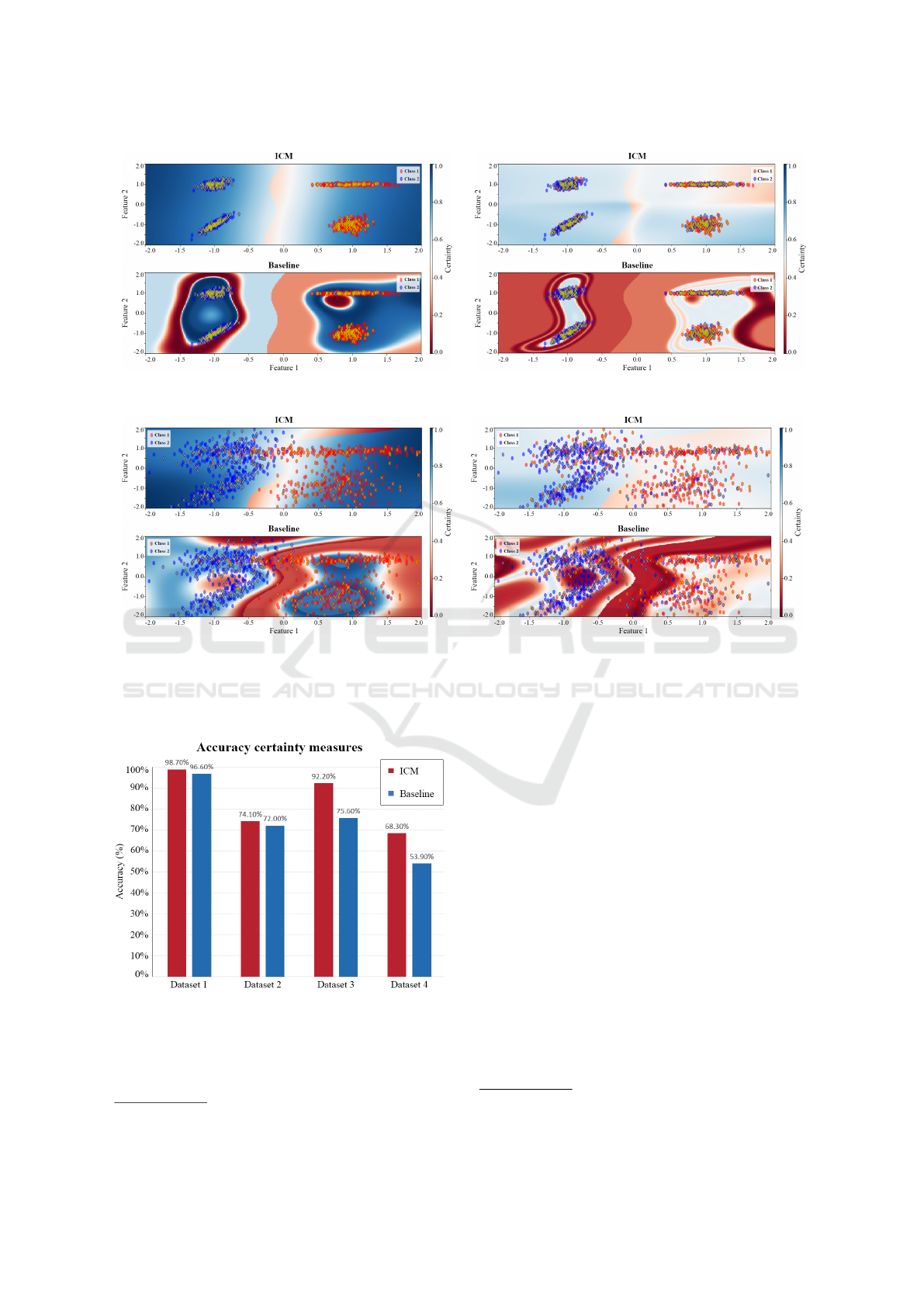
(a) Data set 1, SVM accuracy of 99% and ICM settings of

k = 350, σ

= 0.75, µ

time

= 5 and σ

time

= 1.25

(b) Data set 2, SVM accuracy of 75% and ICM settings of

k = 350, σ

= 0.25, µ

time

= 5 and σ

time

= 1.25

k = 350, σ

= 0.5, µ

time

= 8 and σ

time

= 1.25

(d) Data set 4, SVM accuracy of 72.5% and ICM settings of

k = 350, σ

= 0.5, µ

time

= 8 and σ

time

= 1.25

Figure 1: Each ﬁgure visualizes the certainty values for ICM and of the baseline based on the method from Park et al. (2016).

The point clouds represent the data points from the test set, the yellow points the sampled data points part of M and the

backgrounds represent the certainty values of each of the two approaches.

Figure 2: The accuracy according to equation 4 for both

ICM and the baseline on the four synthetic data sets.

Two years’ worth of data were simulated of which

80% was used to train a neural network and the other

20% was used as a test set

. A neural net with three

The data set is available on request by e-mailing one

hidden layers (1536, 256 and 64 neurons respectively)

was used with ReLu activation functions (Nair and

Hinton, 2010), trained using the ADAM optimizer

(Kingma and Ba, 2015). No attempt was made to

fully optimize the model when it reached an accuracy

of 96.59% with hand tuned hyper-parameters on pre-

dicting three classes 15 minutes in the future; a drift

of < 5m, 5 − 10m or > 10m.

5.2 Results

Figure 3 shows the accuracy of both ICM and the

baseline, calculated according to equation 4. Each

point shows the mean accuracy of twenty different

data sets from the DP test data with varying sample

set sizes. This plot shows that ICM outperforms the

baseline on a high-dimensional data set with a non-

linear machine learning model. The lower accuracies

of the authors. It can be used for other applications and as a

benchmark.

ICM: An Intuitive Model Independent and Accurate Certainty Measure for Machine Learning

319

near chance level, of the baseline and ICM method

on smaller memory sizes is due to both methods not

having enough data with which to learn how to gen-

eralize well. However, ICM is robust to the memory

size as long as this size is above some threshold. For

this speciﬁc problem with high dimensional data and

three classes that size is a mere 20 data points.

Figure 3: The accuracy of the proposed uncertainty measure

compared to the baseline based on the approach by Park et

al. (2016) for various sample set sizes. Accuracy is deter-

mined according to equation 4. The error bars represent the

standard error.

6 CONCLUSION

The goal of this study was to design an intuitive cer-

tainty measure that is widely applicable and accurate.

In this study we deﬁned an intuitive measure as being

based on easily explained and understood principles

that non-experts in machine learning (ML) can under-

stand and that behaves predictable in feature space.

We developed such a measure, the Intuitive Certainty

Measure (ICM), by treating the ML model as a black

box to make it generic and validated its accuracy on

two different ML models of varying complexity.

We designed ICM to be intuitive by basing it on

the notion of distance and previous experiences; if the

output for the current data point is the same as simi-

lar data points experienced in the past, certainty will

be high. This underlying principle is easily explained

such that non-experts can understand the values of

ICM and where they come from. We showed that

ICM acts in a more predictable manner on various two

dimensional synthetic classiﬁcation problems, com-

pared to the baseline.

ICM proved to be accurate; it outputs a high cer-

tainty for the ML model’s true positives and negatives,

while it outputs a low certainty for its false positives

and negatives. It outperformed the baseline method

both on the synthetic classiﬁcation tasks with varying

class separation as well as on a more real-world use-

case with high dimensional data.

Finally, ICM was applied to both support vector

machines and a deep neural network without modi-

ﬁcation. This illustrates that ICM is applicable to a

wide array of machine learning approaches, both lin-

ear as non-linear models. The only requirement is that

it learned a (semi-)supervised problem.

In the future we will validate ICM’s intuitive prop-

erties in a usability study to assess whether ICM in-

deed helps to maintain an appropriate level of trust

in a machine learning based agent. Additional explo-

ration of different sampling methods and the effect of

various distance measures on both accuracy and intu-

itiveness for ICM may result in a broader understand-

ing of the measure. Our future research will result

in a further improved version of ICM that will hope-

fully be both accurate and intuitive for non-experts in

Machine Learning to help manage their trust in their

models.

ACKNOWLEDGMENTS

This study was funded as part of the early re-

search program Human Enhancement within TNO.

The work beneﬁted greatly from the domain knowl-

edge of Ehab el Amam from RH Marine.

REFERENCES

Antol, S., Agrawal, A., Lu, J., Mitchell, M., Batra, D.,

Lawrence Zitnick, C., and Parikh, D. (2015). Vqa:

Visual question answering. In Proc. of the IEEE Int.

Conf. on Computer Vision, pages 2425–2433.

Belard, A., Buchman, T., Forsberg, J., Potter, B. K., Dente,

C. J., Kirk, A., and Elster, E. (2017). Precision diag-

nosis: a view of the clinical decision support systems

(cdss) landscape through the lens of critical care. J.

Clin. Monit. Comput., 31(2):261–271.

Blundell, C., Cornebise, J., Kavukcuoglu, K., and Wierstra,

D. (2015). Weight uncertainty in neural networks.

In Proc. of the 32nd Int. Conf. on Machine Learning

(ICML 2015).

Bottou, L. and Vapnik, V. (1992). Local learning algo-

rithms. Neural computation, 4(6):888–900.

Broekens, J., Harbers, M., Hindriks, K., Van Den Bosch,

K., Jonker, C., and Meyer, J.-J. (2010). Do you get it?

User-evaluated explainable BDI agents. In German

Conf. on Multiagent System Technologies, pages 28–

39. Springer.

Castillo, E., Gutierrez, J. M., and Hadi, A. S. (2012). Expert

systems and probabilistic network models. Springer

Science & Business Media.

ICAART 2018 - 10th International Conference on Agents and Artiﬁcial Intelligence

320

Cohen, M. S., Parasuraman, R., and Freeman, J. T. (1998).

Trust in decision aids: A model and its training impli-

cations. In Proc. Command and Control Research and

Technology Symp. Citeseer.

Core, M. G., Lane, H. C., Van Lent, M., Gomboc, D.,

Solomon, S., and Rosenberg, M. (2006). Building

explainable artiﬁcial intelligence systems. In AAAI,

pages 1766–1773.

Datta, A., Sen, S., and Zick, Y. (2016). Algorithmic trans-

parency via quantitative input inﬂuence: Theory and

experiments with learning systems. In IEEE Symp.

Security and Privacy,, pages 598–617. IEEE.

Dietterich, T. G. and Kong, E. B. (1995). Machine learning

bias, statistical bias, and statistical variance of deci-

sion tree algorithms. Technical report, Dep. of CS.,

Oregon State University.

Dzindolet, M. T., Peterson, S. A., Pomranky, R. A., Pierce,

L. G., and Beck, H. P. (2003). The role of trust

in automation reliance. Int. J. Hum. Comput. Stud.,

58(6):697–718.

Foody, G. M. (2005). Local characterization of thematic

classiﬁcation accuracy through spatially constrained

confusion matrices. Int. J. Remote Sens., 26(6):1217–

1228.

Giarratano, J. C. and Riley, G. (1998). Expert systems. PWS

Publishing Co.

Harrington, P. (2012). Machine learning in action, vol-

ume 5. Manning Greenwich, CT.

Kingma, D. and Ba, J. (2015). Adam: A method for

stochastic optimization. 3rd Int. Conf. for Learning

Representations.

Langley, P., Meadows, B., Sridharan, M., and Choi, D.

(2017). Explainable Agency for Intelligent Au-

tonomous Systems. In AAAI, pages 4762–4764.

Nair, V. and Hinton, G. E. (2010). Rectiﬁed linear units

improve restricted boltzmann machines. In Proc. of

the 27th Int. Conf. on Machine Learning (ICML-10),

pages 807–814.

Nguyen, A., Yosinski, J., and Clune, J. (2015). Deep neural

networks are easily fooled: High conﬁdence predic-

tions for unrecognizable images. In Proc. of the IEEE

Conf. on Computer Vision and Pattern Recognition,

pages 427–436.

Norton, S. W. (2013). An explanation mechanism for

bayesian inferencing systems. In Proc. of the 2nd

Conf. on Uncertainty in Artiﬁcial Intelligence.

Park, N.-W., Kyriakidis, P. C., and Hong, S.-Y. (2016). Spa-

tial estimation of classiﬁcation accuracy using indi-

cator kriging with an image-derived ambiguity index.

Remote Sensing, 8(4):320.

Platt, J. et al. (1999). Probabilistic outputs for support

vector machines and comparisons to regularized like-

lihood methods. Adv. in large margin classiﬁers,

10(3):61–74.

Raaijmakers, S., Sappelli, M., and Kraaij, W. (2017). Inves-

tigating the interpretability of hidden layers in deep

text mining. In Proc. of SEMANTiCS.

Ribeiro, M. T., Singh, S., and Guestrin, C. (2016a). Nothing

Else Matters: Model-Agnostic Explanations By Iden-

tifying Prediction Invariance.

Ribeiro, M. T., Singh, S., and Guestrin, C. (2016b). Why

should i trust you?: Explaining the predictions of

any classiﬁer. In Proc. of the 22nd ACM SIGKDD

Int. Conf. on Knowledge Discovery and Data Mining,

pages 1135–1144. ACM. arXiv: 1602.04938.

Rippa, S. (1999). An algorithm for selecting a good value

for the parameter c in radial basis function interpola-

tion. Adv. Comput. Math., 11(2):193–210.

Saelid, S., Jenssen, N., and Balchen, J. (1983). Design

and analysis of a dynamic positioning system based

on kalman ﬁltering and optimal control. IEEE Trans.

Autom. Control, 28(3):331–339.

Schaefer, K. E., Straub, E. R., Chen, J. Y., Putney, J., and

Evans, A. W. (2017). Communicating Intent to De-

velop Shared Situation Awareness and Engender Trust

in Human-Agent Teams. Cognit. Syst. Res.

Sch

olkopf, B., Sung, K.-K., Burges, C. J., Girosi, F.,

Niyogi, P., Poggio, T., and Vapnik, V. (1997). Com-

paring support vector machines with gaussian kernels

to radial basis function classiﬁers. IEEE Trans. Signal

Process., 45(11):2758–2765.

Selvaraju, R. R., Das, A., Vedantam, R., Cogswell, M.,

Parikh, D., and Batra, D. (2016). Grad-cam: Why

did you say that? visual explanations from deep net-

works via gradient-based localization. arXiv preprint

arXiv:1610.02391.

Silver, D., Huang, A., Maddison, C. J., Guez, A., Sifre, L.,

Van Den Driessche, G., Schrittwieser, J., Antonoglou,

I., Panneershelvam, V., Lanctot, M., et al. (2016).

Mastering the game of go with deep neural networks

and tree search. Nature, 529(7587):484–489.

Swartout, W., Paris, C., and Moore, J. (1991). Explanations

in knowledge systems: Design for explainable expert

systems. IEEE Expert., 6(3):58–64.

van Diggelen, J., van den Broek, H., Schraagen, J. M., and

van der Waa, J. (2017). An intelligent operator support

system for dynamic positioning. In Int. Conf. on Ap-

plied Human Factors and Ergonomics, pages 48–59.

Springer.

Vidovic, M. M.-C., Grnitz, N., Mller, K.-R., and Kloft, M.

(2016). Feature Importance Measure for Non-linear

Learning Algorithms. arXiv:1611.07567 [cs, stat].

arXiv: 1611.07567.

Wettschereck, D., Aha, D. W., and Mohri, T. (1997). A

review and empirical evaluation of feature weighting

methods for a class of lazy learning algorithms. In

Lazy learning, pages 273–314. Springer.

ICM: An Intuitive Model Independent and Accurate Certainty Measure for Machine Learning

321