Automated Diagnosis of Breast Cancer and Pre-invasive Lesions on

Digital Whole Slide Images

Ezgi Mercan

, Sachin Mehta

, Jamen Bartlett

, Donald L. Weaver

, Joann G. Elmore

and Linda G. Shapiro

Paul G. Allen School of Computer Science and Engineering, University of Washington, Seattle, WA, U.S.A.

Department of Electrical Engineering, University of Washington, Seattle, WA, U.S.A.

Department of Pathology, University of Vermont, Burlington, VT, U.S.A.

Deparment of Medicine, University of Washington, Seattle, WA, U.S.A.

Keywords:

Breast Pathology, Automated Diagnosis, Histopathological Image Analysis.

Abstract:

Digital whole slide imaging has the potential to change diagnostic pathology by enabling the use of computer-

aided diagnosis systems. To this end, we used a dataset of 240 digital slides that are interpreted and diagnosed

by an expert panel to develop and evaluate image features for diagnostic classiﬁcation of breast biopsy whole

slides to four categories: benign, atypia, ductal carcinoma in-situ and invasive carcinoma. Starting with a

tissue labeling step, we developed features that describe the tissue composition of the image and the struc-

tural changes. In this paper, we ﬁrst introduce two models for the semantic segmentation of the regions of

interest into tissue labels: an SVM-based model and a CNN-based model. Then, we deﬁne an image feature

that consists of superpixel tissue label frequency and co-occurrence histograms based on the tissue label seg-

mentations. Finally, we use our features in two diagnostic classiﬁcation schemes: a four-class classiﬁcation,

and an alternative classiﬁcation that is one-diagnosis-at-a-time starting with invasive versus benign and ending

with atypia versus ductal carcinoma in-situ (DCIS). We show that our features achieve competitive results

compared to human performance on the same dataset. Especially at the critical atypia vs. DCIS threshold, our

system outperforms pathologists by achieving an 83% accuracy.

1 INTRODUCTION

The importance of early detection in breast can-

cer is well understood and has been emphasized for

decades. Today, regular screenings for certain pop-

ulations are recommended and conducted especially

in developed countries. However, there is a grow-

ing concern in the medical community that the fear

of under-diagnosing a patient leads to over-diagnosis

and contributes to the ever-increasing number of pre-

invasive and invasive cancer cases. Recent ﬁndings

indicate that DCIS cases might be over-treated with-

out signiﬁcantly better outcomes, making diagnostic

errors even more critical for patient care (Park et al.,

2017). Diagnostic errors are alarmingly high, espe-

cially for pre-invasive lesions of the breast. A recent

study showed that the agreement between patholo-

gists and experts for the atypia cases is only 48% (El-

more et al., 2015).

Digital whole slide imaging provides researchers

with an opportunity to study the diagnostic errors and

(a) benign (b) atypia (c) DCIS (d) invasive

cancer

Figure 1: Example images from four diagnostic categories

of our dataset.

develop image features for accurate and efﬁcient di-

agnosis. An automated diagnosis system can assist

pathologists by highlighting diagnostically relevant

regions and image features associated with the malig-

nancy, therefore providing unbiased and reproducible

feedback. The success of a diagnostic support sys-

tem depends on the descriptive power of the image

features considering the complexity that the full spec-

trum of diagnoses that the breast biopsies present.

The majority of breast cancers are ductal, i.e.

cancer of the breast ducts. The breast ducts are

Mercan, E., Mehta, S., Bartlett, J., Weaver, D., Elmore, J. and Shapiro, L.

Automated Diagnosis of Breast Cancer and Pre-invasive Lesions on Digital Whole Slide Images.

DOI: 10.5220/0006550600600068

In Proceedings of the 7th International Conference on Pattern Recognition Applications and Methods (ICPRAM 2018), pages 60-68

ISBN: 978-989-758-276-9

pipe-like structures that are responsible for produc-

ing and delivering the milk. Breast biopsies are two-

dimensional cross-sections of the breast tissue, and a

healthy duct appears as a circular arrangement of two

layers of epithelial cells. These cells can proliferate

in different degrees and change the structure of the

ducts. The diagnosis of the biopsy depends on the

correct interpretation of these cellular and structural

changes. Figure 1 shows example breast biopsy im-

ages from our dataset with different diagnoses, that

range from benign tissue to invasive cases.

We propose an automated diagnosis system for

breast tissue using digital whole slides images (WSIs)

of breast biopsies. To this end, we used a dataset of

breast WSIs with a wide range of diagnoses from be-

nign to invasive cancer. The ﬁrst step of our diagnosis

pipeline is the semantical segmentation of biopsy im-

ages into different tissues. We then extracted features

from the semantic masks that describe the distribution

and arrangement of the tissue in the image. Finally,

we trained classiﬁers with our tissue-label-based fea-

tures for automated diagnosis of the biopsy images.

Our experimental results suggest that the features ex-

tracted from the semantic masks have high descriptive

power and helps in differentiating a wide range of di-

agnoses, from benign to invasive.

Our work on automated diagnosis of breast biopsy

images considers the full spectrum of diagnoses en-

countered in clinical practice. We designed a novel

semantic segmentation scheme with a set of tissue

labels developed for invasive cancer as well as pre-

invasive lesions of the breast. The semantic seg-

mentation gives us a powerful abstraction for diag-

nostic classiﬁcation, so that even simple features ex-

tracted from the segmentation masks can achieve re-

sults comparable to the diagnostic accuracy of the ac-

tual pathologists.

2 RELATED WORK

Automated Diagnosis. Automated malignancy de-

tection is a well-studied area in the histopathological

image analysis literature. Most of the related work

focuses on the detection of cancer in a binary classi-

ﬁcation setting with only malignant and benign cases

(Chekkoury et al., 2012; Doyle et al., 2012; Tabesh

et al., 2007). These methods do not take pre-invasive

lesions or other diagnostic categories into account,

which limits their use in real-world scenarios. There

is also limited research on analyzing images for sub-

type classiﬁcation (Kothari et al., 2011) or stromal de-

velopment (Sertel et al., 2008) using only tumor im-

ages.

Recently, some researchers have begun to study

the pre-invasive lesions of the breast: (Dong et al.,

2014) reports promising results in discrimination of

benign proliferations of the breast from malignant

ones. They extract 392 features corresponding to

the mean and standard deviation in nuclear size and

shape, intensity and texture across 8 color channel,

and apply L1-regularized logistic regression to build

discriminative models. Their dataset contains only

usual ductal hyperplasia (UDH), which maps to be-

nign in our dataset, and ductal carcinoma in-situ

(DCIS) cases. To our best knowledge, there is no

study that considers the full spectrum of pre-invasive

lesions of the breast including atypia (atypical duc-

tal hyperplasi and atypical lobular hyperplasia). Our

study is the ﬁrst of its kind to attempt a diagnostic

classiﬁcation with categories from benign to invasive

cancer.

CNNs for Medical Image Analysis. Convolutional

neural networks (CNNs) have been successfully ap-

plied for medical image analysis. Most notable

among is: classifying WSI into tumor subtypes and

grades (Hou et al., 2016), segmenting EM images

(Ronneberger et al., 2015), segmenting gland im-

ages (Chen et al., 2017), and segmenting brian im-

ages (Fakhry et al., 2017). (Hou et al., 2016) apply

a sliding-window approach to reduce the WSI size

and combine predictions made on patches to classify

WSIs. Their work exploits WSI characteristics such

as the heterogeneity of tissue in terms of tumor grades

and subtypes. (Ronneberger et al., 2015), (Chen et al.,

2017), and (Fakhry et al., 2017) follow an encoder-

decoder network approach with skip-connections for

segmenting medical images. For semantic segmenta-

tion using CNN, we use the recently proposed resid-

ual encoder-decoder network by (Fakhry et al., 2017).

3 DATASET

3.1 Breast Biopsy Whole Slide Images

240 breast biopsies were selected from the Breast

Cancer Surveillance Consortium (http://www.bcsc-

research.org/) archives in New Hampshire and Ver-

mont for our studies. The ﬁnal dataset spans a wide

spectrum of breast diagnoses that are mapped to four

categories: benign, atypia, ductal carcinoma in-situ

(DCIS) and invasive cancer.

The original H&E (heamatoxylin and eosin)

stained glass slides were scanned to produce whole

slide images using an iScan CoreoAu



in 40X mag-

niﬁcation. Quality control was conducted by a tech-

Automated Diagnosis of Breast Cancer and Pre-invasive Lesions on Digital Whole Slide Images

Table 1: Distribution of the diagnostic categories based on

expert consensus.

Diagnostic Category # of Cases # of ROIs

Benign 60 102

Atypia 80 128

DCIS 78 162

Invasive cancer 22 36

Total 240 428

nician and an experienced breast pathologist to obtain

the highest quality. The ﬁnal average image size for

the 240 digital slides was 90,000 × 70,000 pixels.

3.2 Expert Consensus Diagnoses and

Regions of Interest

Each digital slide was ﬁrst interpreted and diagnosed

by three expert pathologists individually. Each ex-

pert provided a diagnosis and a region of interest

(ROI) that supports the diagnosis for each digital

slide. Following the individual interpretations, sev-

eral in-person and webinar meetings were held to pro-

duce an expert-consensus diagnosis and one or more

expert consensus ROIs for each case. Since some

cases had more than one ROI per WSI, the ﬁnal set

of expert consensus ROIs includes 102 benign, 128

atypia, 162 DCIS and 36 invasive samples. Table 1

summarizes the data. For a detailed explanation of

the development of the cases and the expert consen-

sus data, please see (Oster et al., 2013) and (Allison

et al., 2014).

3.3 Tissue Labels

To describe the structural changes that lead to can-

cer in the breast tissue, we produced a set of eight

tissue labels in collaboration with an expert patholo-

gist: background, benign epithelium, malignant ep-

ithelium, normal stroma, desmoplastic stroma, secre-

tion, blood, and necrosis.

The epithelial cells in the benign and atypia cat-

egories were labeled as benign epithelium, whereas

the epithelial cells from the DCIS and invasive can-

cer categories were labeled with the malignant ep-

ithelium label. Compared to benign cells, the cells in

the malignant epithelium are bigger and irregular in

shape. Stroma is a term used for the connective tissue

between the ductal structures in the breast. In some

cases, stromal cells proliferate in response to cancer.

We used desmoplastic stroma and normal stroma la-

bels for the stroma associated with the tumor and reg-

ular breast stroma, respectively. Since breast ducts

are glands responsible for producing the milk, they

are sometimes ﬁlled with molecules discharged from

the cells. The secretion label was used to mark this

benign substance ﬁlling the ducts. The label necrosis

was used to mark the dead cells at the center of the

ducts in the DCIS and invasive cases. The blood label

was used to mark the blood cells, which are rare but

have a very distinct appearance. Finally, the pixels

that do not contain any tissue, including the empty

areas inside the ducts, were labeled as background.

Figure 2 illustrates the eight tissue labels marked by

the pathologist.

Although some of the labels are not important in

diagnostic interpretation, our tissue labels were in-

tended to cover all the pixels in the images. Due to

the expertise needed for labeling and the large sizes of

the WSIs, we randomly selected a subset of 40 cases

(58 ROIs). These 58 ROIs are annotated by a pathol-

ogist into eight tissue labels. Figure 2. shows three

example images and the pixel labels provided by a

pathologist.

4 METHODOLOGY

4.1 Semantic Segmentation

Segmenting WSIs of breast biopsies into building

blocks is crucial to understand the structural changes

that lead to diagnosis. Semantic segmentation masks

can provide important information about the distribu-

tion and arrangement of different tissue types.

We used a supervised machine learning approach

to semantically segment H&E images into eight tis-

sue labels. We trained and evaluated two models:

(1) an SVM-based model that starts with a super-

pixel segmentation and assigns each superpixel a tis-

sue label based on color and texture features, and (2)

a CNN-based model with a sliding-window approach

that classiﬁes each pixel in a sliding-window into a

background

benign epithelium

malignant epithelium

normal stroma

desmoplastic stroma

secretion

blood necrosis

Figure 2: The set of tissue labels used in semantic segmen-

tation: (top row) three example cases from the dataset and

(bottom row) the pixel labels provided by a pathologist.

ICPRAM 2018 - 7th International Conference on Pattern Recognition Applications and Methods

label class simultaneously.

4.1.1 Segmentation using SVM

We used the SLIC algorithm (Achanta et al., 2012) to

segment H&E images into superpixels of size 3000

pixel. From each superpixel, we extracted L*a*b*

color histograms and LBP texture histograms (He and

Wang, 1990). We calculated the texture histograms

from the H&E channels, which were obtained through

a color deconvolution algorithm (Ruifrok and John-

ston, 2001).

The size of the superpixels, 3,000 pixels, was se-

lected to have approximately one or two epithelial

cells in one superpixel so that the detailed structures

of the ducts could be captured. Our preliminary ex-

periments showed that some individual superpixels

were misclassiﬁed, while their neighbors were cor-

rectly classiﬁed. To improve the classiﬁcation, we

included two circular neighborhoods around each su-

perpixel in feature extraction. The color and texture

histograms calculated from the superpixels and circu-

lar neigborhoods were concatenated to produce one

feature vector for each superpixel. Figure 3 illustrates

the two circular neighborhoods from which the same

features were extracted and appended to superpixel

feature vector.

(a) superpixel segmentation (b) neighborhoods

Figure 3: Initial superpixel segmentation and the circular

neighborhoods used to increase the superpixel classiﬁcation

accuracy for supervised segmentation.

We used the concatenated color and texture his-

tograms to train an SVM model that classiﬁes super-

pixels into eight tissue labels. To address the non-

uniform distribution of the tissue labels and ROI size

variation, we sampled 2000 superpixels for each of

the eight labels (if possible) from each ROI. We eval-

uated the performance of the SVM-based model in

10-fold cross-validation experiments on the subset of

ROIs labeled by the pathologist (N=58). For the di-

agnostic classiﬁcation, we trained a ﬁnal SVM model

with the samples from all folds and applied the model

to the full dataset (N=428 ROIs) to obtained tissue la-

bel segmentations.

4.1.2 Segmentation using CNN

The CNN experiments were an attempt to improve

the semantic segmentation performance achieved by

the feature-based SVM methodology. Rather than us-

ing features, the CNN learns to recognize the patterns

from the image itself. Following the work of (Fakhry

et al., 2017), we implemented a residual encoder-

decoder network. The encoding network transforms

an input image into a feature vector space by stack-

ing a series of encoding blocks. The decoding net-

work transforms the feature vector space into a se-

mantic mask by stacking a series of decoding blocks.

The residual connection between the encoding and its

corresponding decoding block give chance to each in-

termediate block to represent the information inde-

pendent of the blocks at any other spatial level. See

(Mehta et al., 2017) for more details about the CNN

network.

We split 58 ROIs into training (30 ROIs) and test

(28 ROIs) sets keeping the distribution of diagnos-

tic categories similar. We used a sliding-window

approach to create samples for training and testing

the CNN architecture. We cropped 256 × 256 pixel

patches at different resolutions, resulting in 5,312

patches from 30 ROIs. We augmented the data using

random rotations (between 5 and 10 degree), horizon-

tal ﬂips, and random crops followed by scaling (i.e.

the crop border was selected randomly between 20

and 50 pixels), resulting in a total of 25,992 patches

that were split into the training and validation sets us-

ing 90:10 split ratio. We trained all of our models end-

to-end using stochastic gradient descent with a ﬁxed

learning rate of 0.0001, momentum of 0.9, weight

decay of 0.0005, and a batch size of 10 on a single

NVIDIA GTX-1080 GPU.

4.2 Tissue Label Frequency and

Co-occurrence Histograms

One of the basic visual differences between diagnos-

tic categories is the existence and amount of different

tissue types. To this end, we calculated frequency his-

tograms for the superpixel labels. However, only the

distribution of the tissue types is not enough to de-

scribe complex spatial relationships. Co-occurrence

histograms, on the other hand, can capture the fre-

quency of the contact between the superpixels with

different tissue labels.

We normalized all histograms to remove the effect

of the size. Since the background was one of the tis-

sue labels, the amount of background affects the his-

togram bins of other tissue types, yet the amount of

background may not be important in diagnostic clas-

Automated Diagnosis of Breast Cancer and Pre-invasive Lesions on Digital Whole Slide Images

siﬁcation. We created and studied two alternative ver-

sions to all features by removing the background bin,

and then also removing the stroma bin from the his-

tograms before normalization.

4.3 Diagnostic Classiﬁcation

The diagnostic decision making process is complex.

Pathologists interpret the slides at different resolu-

tions and make decisions about different diagnoses.

For example, the decision to diagnose an invasive car-

cinoma is usually made at a lower resolution, where

a high-level organization of the tissue is available to

the observer. On the other hand, the decision between

atypia and DCIS is made at a higher resolution by ex-

amining structural and cellular changes. Inspired by

this observation, we designed a classiﬁcation scheme

where a decision is made for one diagnosis at a time.

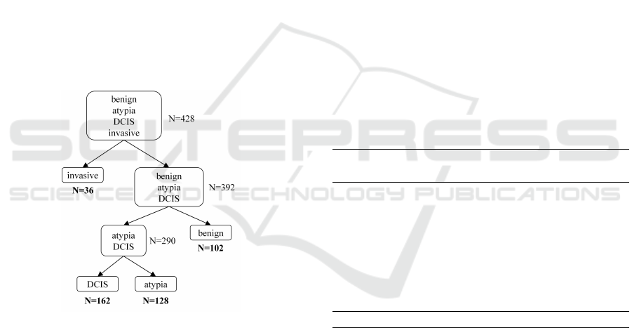
We designed a set of experiments to test two diag-

nostic classiﬁcation schemes: (1) A model that classi-

ﬁes an ROI into one of the four diagnostic categories,

and (2) a model that eliminates one diagnosis at a time

(Figure 4).

Figure 4: One-diagnosis-at-a-time classiﬁcation.

In diagnostic classiﬁcation experiments, we used

all expert consensus ROIs (N=428) as described in

Section 3.1. For the 4-diagnosis classiﬁcation, we

trained an SVM using all samples. For the sec-

ond classiﬁcation scheme (Figure 4), we trained three

SVMs: 1) invasive vs. not-invasive, using all sam-

ples; 2) atypia and DCIS vs. benign, using benign,

atypia and DCIS samples; 3) DCIS vs. atypia, using

atypia and DCIS samples. When the sample size was

smaller than the number of features, we applied prin-

cipal components analysis (PCA) and used the ﬁrst

20 principal components to reduce the number of fea-

tures. For all experiments, we trained SVMs in a 10-

fold cross-validation setting using each ROI separa-

tely as a sample. We sub-sampled the training data

to have an equal number of samples for each class.

To remove the effect of sub-sampling, we repeated all

experiments 100 times and reported the average accu-

racies.

5 RESULTS

We evaluated both the tissue label segmentation and

diagnostic classiﬁcation tasks. Note that any error

produced by the segmentation is propagated to the di-

agnostic classiﬁcation, since the features used for di-

agnosis are based on tissue labels.

5.1 Tissue Label Segmentation

We evaluated the performances of the SVM method

and the CNN method by comparing the predicted

pixel labels with the ground truth pixel labels pro-

vided by the pathologist. We report precision and re-

call metrics for both models on the test set of 20 ROIs

in Table 2 and confusion matrices in Figure 5.

Table 2: Tissue label segmentation results: Individual label

and average precision and recall values for the SVM-based

and CNN-based supervised segmentations.

Precision Recall

Tissue Label SVM CNN SVM CNN

background .86 .81 .89 .93

benign epi .23 .39 .46 .72

malignant epi .63 .86 .48 .61

normal stoma .68 .28 .24 .88

desm. stroma .63 .72 .61 .20

secretion .01 .32 .24 .49

necrosis .03 .09 .24 .59

blood .35 .52 .46 .83

Average .43 .50 .45 .66

The CNN model performed better than the SVM

method in every label, other than the desmoplastic

stroma label. The CNN method performed especially

well with the rare labels of secretion, blood and necro-

sis with high precision and recall values. However, it

suffers from a low precision, high recall of the nor-

mal stroma label. This may be due to predicting the

majority of the desmoplastic stroma pixels as normal

stroma (See Figure 5).

5.2 Diagnostic Classiﬁcation

Table 3 shows the average accuracy, (t p +tn)/(t p +

tn + f p + f n), sensitivity, t p/(t p + f n), and speci-

ﬁcity, tn/(tn + f p), values for the three variations of

ICPRAM 2018 - 7th International Conference on Pattern Recognition Applications and Methods

background

benign epi

malignant epi

normal

strm

desmopl

strm

secretion

necrosis

blood

Prediction

background

benign epi

malignant epi

normal

strm

desmopl

strm

secretion

necrosis

blood

Prediction

background

Ground Truth

benign epi

malignant epi

normal

strm

desmopl

strm

secretion

necrosis

blood

.89

.01

.00

.02

.07

.01

.00

.01

.46

.36

.01

.08

.03

.04

.00

.02

.12

.48

.00

.22

.15

.00

.04

.01

.06

.24

.42

.18

.02

.03

.04

.03

.17

.03

.61

.11

.01

.00

.13

.02

.07

.18

.16

.24

.08

.13

.12

.04

.13

.00

.26

.20

.24

.01

.03

.01

.05

.13

.23

.05

.04

.46

.93

.01

.03

.01

.00

.01

.72

.16

.09

.01

.00

.06

.09

.61

.13

.07

.02

.03

.00

.03

.02

.01

.88

.05

.00

.01

.06

.02

.05

.66

.20

.00

.01

.15

.06

.05

.07

.02

.49

.09

.07

.10

.01

.11

.01

.15

.59

.01

.10

.04

.00

.83

(a) SVM (b) CNN

Figure 5: Confusion matrices for both SVM-based and

CNN-based models for the eight-label semantic segmenta-

tion task on 20 test ROIs.

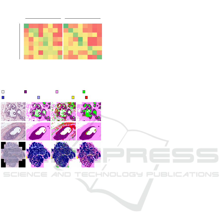
background

benign epithelium

malignant epithelium

normal stroma

desmoplastic stroma

secretion

blood necrosis

(a) RGB (b) Ground (c) SVM (d) CNN

Truth

Figure 6: Visualizations of the segmentations produced by

the SVM and CNN using the eight tissue labels: (a) input

image, (b) ground truth labels, (c) the prediction of the SVM

model, (d) the prediction of the CNN model.

tissue label frequency and co-occurrence histograms

with two different segmentation techniques in four

classiﬁcation tasks, where t p is the number of true

positives, f p is the number of false positives, tn is

the number of true negatives, and f n is the number

of false negatives. Although accuracy is the more

common metric for evaluating classiﬁcation perfor-

mance, sensitivity and speciﬁcity are two metrics that

are widely used in the evaluation of diagnostic tests.

They measure the true positive and true negative rates

of a condition. Sensitivity quantiﬁes the absence of

false negatives, while speciﬁcity quantiﬁes the ab-

sence of false positives. Since our dataset is unbal-

anced for different diagnostic classes, we report the

sensitivity and speciﬁcity metrics to illustrate the per-

formance of our automated diagnosis experiments.

The four-class classiﬁcation setting obtains a max-

imum of 0.46 accuracy using all tissue labels with the

CNN-based segmentation. In comparison, one-

diagnosis-at-a-time setting achieves accuracies of

0.94, 0.70 and 0.83 for the differentiation of invasive,

benign and DCIS respectively.

The accuracies are higher for the CNN-based seg-

mentation method as expected, except for the differ-

entiation of atypia and DCIS from benign. However,

the sensitivity and speciﬁcity for the experiment with

all tissue labels with SVM-based segmentation are not

as high as the other experiments. The experiment with

no background or stroma with CNN-based segmenta-

tion achieves higher sensitivity (0.94) and speciﬁcity

(0.39) despite the low accuracy value (0.60). This is

likely due to the class imbalance between the benign

and non-benign samples.

Removing the background label improves the dif-

ferentiation of invasive from non-invasive lesions;

however, removing the stroma label results in lower

accuracy. The best result for differentiation of inva-

sive is achieved with tissue labels with no background

using CNN-based segmentation. Removing both the

background and stroma labels improves the accuracy

of classiﬁcation DCIS vs. atypia. Tissue label his-

tograms with no background or stroma with CNN-

based segmentation achieves accuracy of 0.83, sen-

sitivity of 0.88 and speciﬁcity of 0.78.

6 DISCUSSION

SVM vs CNN for Segmentation

The CNNs outperformed many of the traditional mod-

els composed of a classiﬁer and hand-crafted image

features in classiﬁcation, detection and segmentation

tasks. Our experiments showed that it is possible

to obtain a performance boost by using an encoder-

decoder architecture speciﬁcally designed for the

breast biopsy images. Although the improvement

seems small, the contribution of CNNs was in the

classes of necrosis, epithelium and stroma, which are

important for distinguishing and classifying DCIS.

The differentiation between necrosis and secretion

might be especially critical in diagnosis.

Furthermore, none of the quantitative measure-

ments evaluated the smooth object boundaries ob-

tained by the CNNs. Because the CNN-based meth-

ods were trained with patches that are 500 times big-

ger than a superpixel, they were able to learn the

structure and segment smooth borders of the objects

as it can be seen in visualizations in Figure 6.

Automated Diagnosis of Breast Cancer and Pre-invasive Lesions on Digital Whole Slide Images

Table 3: Comparison of features with different tissue histograms and segmentations for the diagnostic classiﬁcation tasks.

Accuracy Sensitivity Speciﬁcity

Tissue Labels SVM CNN SVM CNN SVM CNN

4-class

All labels .32 .46 - - - -

No background .39 .44 - - - -

No background or stroma .33 .42 - - - -

Invasive vs. Benign-Atypia-DCIS

All labels .48 .82 .13 .24 .97 .95

No background .62 .94 .15 .70 .97 .95

No background or stroma .54 .69 .12 .17 .96 96

Atypia-DCIS vs. Benign

All labels .70 .51 .79 .88 .41 .33

No background .65 .43 .80 .94 .37 .31

No background or stroma .69 .60 .83 .94 .42 .39

DCIS vs. Atypia

All labels .68 .71 .73 .67 .63 .93

No background .65 .78 .62 .75 .92 .85

No background or stroma .72 .83 .70 .88 .76 .78

Importance of Stroma in Diagnosis

When the stroma label was not used in feature calcu-

lations, the accuracy for the classiﬁcation of invasive

cases dropped indicating the importance of stroma in

differentiation of breast tumors. By encoding two dif-

ferent types of stroma, we incorporated an important

visual cue used by pathologists when diagnosing in-

vasive carcinomas. Our ﬁndings are consistent with

the existing literature that showed the importance of

stroma not only in diagnosis, but also in the prediction

of survival time (Beck et al., 2011).

Similarly, removing stroma bins from the his-

tograms did not improve the classiﬁcation of the

atypia and DCIS cases from the benign proliferations;

however, the difference was not signiﬁcant in better

performing SVM-segmented features.

Removing stroma improved the classiﬁcation ac-

curacy between DCIS and atypia, as expected. Since

both lesions are mostly restricted to ductal structures

and the diagnosis is made using cellular features and

the degree of structural changes in the ducts, the most

important feature for this task was the epithelial tis-

sue labels and their frequency and co-occurrence with

other labels. It is likely that removing stroma acted as

a noise ﬁltering (or reduction); thereby learning more

relevant features.

Atypia vs. DCIS

Automated diagnosis of pre-invasive lesions of breast

is an understudied problem mostly due to the lack

of comprehensive datasets and difﬁculty of the prob-

lem. The differentiation between DCIS, atypical pro-

liferations and benign proliferations is a hard prob-

lem even for humans, yet the distinction between

two categories could alter the treatment of the patient.

Although both diagnoses are associated with higher

risks of developing invasive breast cancer, it is not

uncommon to treat high grade DCIS cases with oral

chemotherapy and even surgery while atypia cases

are usually followed up with additional screenings.

Features based on frequency and co-occurence his-

tograms of tissue labels were able to capture the vi-

sual characteristics of the breast tissue and achieved

good results.

In a previous study, a group of pathologists inter-

preted slides of breast biopsies (Elmore et al., 2015).

The calculated accuracies from the provided confu-

sion matrix are 70%, 98%, 81% and 80% for the tasks

of 4-class, Invasive vs. Benign-Atypia-DCIS, Atypia-

DCIS vs. Benign and DCIS vs. Atypia respectively.

For the same task, our fully automated pipeline accu-

racies are comparable to the actual pathologists. Our

method outperform the pathologists by 3% on the task

of differentiating DCIS from atypia cases.

ICPRAM 2018 - 7th International Conference on Pattern Recognition Applications and Methods

Sensitivity and Speciﬁcity

The classiﬁer achieves a high accuracy (94%) for the

differentiation of invasive cases from non-invasive le-

sions (benign, atypia and DCIS). For this setting,

relatively low sensitivity (70%) and high speciﬁcity

(95%) indicates that the classiﬁer model is produc-

ing more false negatives than false positives. In other

words, the automated system is somewhat under-

diagnosing for the invasive cancer. This might be due

to the limited number of invasive cases in our dataset

in comparison to other diagnostic classes. Further-

more, the invasive samples include some difﬁcult-to-

differentiate cases like micro-invasions. Also, auto-

mated cancer detection is a well-studied problem in

which researchers setup a binary classiﬁcation prob-

lem with invasive cases and non-invasive cases. Our

contribution in this work is the exploration of pre-

invasive lesions of breast in automated diagnosis set-

ting.

The high sensitivity (79%) and low speciﬁcity

(41%) values for the classiﬁcation of atypia-DCIS and

benign indicates, on the other hand, a clear overdiag-

nosis. This is not as alarming as an underdiagnosis in

the scope of a computer aided diagnosis tool, consid-

ering an overdiagnosed benign case can be caught by

the pathologist and corrected.

Finally, for the DCIS vs. atypia task, our classiﬁer

achieves very good sensitivity and speciﬁcity scores,

88% and 78%, respectively.

7 CONCLUSIONS

We aimed to develop image features that can describe

the diagnostically important visual characteristics of

the breast biopsy images. We took an approach that is

motivated by the pathologists’ decision making pro-

cess. We ﬁrst segment images into eight tissue types

that we determined important for the diagnosis using

two different methods: an SVM-based approach that

uses color and texture features to classify superpix-

els to produce a tissue labeling, and a CNN-based ap-

proach that uses raw images. Then we calculate tissue

label frequency and co-occurrence histograms based

on superpixel segmentation to classify images into

diagnostic categories. In classiﬁcation, we compare

two schemes: we train an SVM classiﬁer to classify

images into four diagnostic categories and we train

a series of SVM classiﬁers to classify images one-

diagnosis-at-a-time. Our proposed one-diagnosis-at-

a-time strategy proved to be more accurate, since it

allows classiﬁer to learn different features for differ-

ent diagnostic categories.

Our strategy of diagnosis by elimination is in-

spired by the diagnostic decision making process of

pathologists and it produced comparable accuracies to

humans. Especially at the border of DCIS and atypia,

our features achieve an accuracy of 83% which is 3%

higher than that of pathologists reported on the same

dataset.

We implemented the simple tissue label frequency

and co-occurrence features to demonstrate the power

of semantic segmentation in diagnosing breast can-

cer. Our ongoing work focuses on developing more

sophisticated features based on tissue labels that can

capture the speciﬁc structural changes in the breast.

ACKNOWLEDGEMENTS

Research reported in this publication was sup-

ported by the National Cancer Institute awards R01

CA172343, R01 CA140560 and RO1 CA200690.

The content is solely the responsibility of the authors

and does not necessarily represent the views of the

National Cancer Institute or the National Institutes

of Health. We thank Ventana Medical Systems, Inc.

(Tucson, AZ, USA), a member of the Roche Group,

for the use of iScan Coreo Au

whole slide imaging

system, and HD View SL for the source code used to

build our digital viewer. For a full description o f HD

View SL, please see http://hdviewsl.codeplex.com/.

REFERENCES

Achanta, R., Shaji, A., Smith, K., Lucchi, A., Fua, P., and

usstrunk, S. (2012). SLIC superpixels compared to

state-of-the-art superpixel methods. IEEE Transac-

tions on Pattern Analysis and Machine Intelligence,

34(11):2274–2281.

Allison, K. H., Reisch, L. M., Carney, P. A., Weaver, D. L.,

Schnitt, S. J., O’Malley, F. P., Geller, B. M., and El-

more, J. G. (2014). Understanding diagnostic variabil-

ity in breast pathology: lessons learned from an expert

consensus review panel. Histopathology, 65(2):240–

251.

Beck, A. H., Sangoi, A. R., Leung, S., Marinelli, R. J.,

Nielsen, T. O., van de Vijver, M. J., West, R. B., van de

Rijn, M., and Koller, D. (2011). Systematic analy-

sis of breast cancer morphology uncovers stromal fea-

tures associated with survival. Science Translational

Medicine, 3(108):108ra113–108ra113.

Chekkoury, A., Khurd, P., Ni, J., Bahlmann, C., Kamen, A.,

Patel, A., Grady, L., Singh, M., Groher, M., Navab,

N., Krupinski, E., Johnson, J., Graham, A., and We-

instein, R. (2012). Automated malignancy detection

in breast histopathological images. In SPIE Medi-

cal Imaging, volume 8315, page 831515. International

Society for Optics and Photonics.

Automated Diagnosis of Breast Cancer and Pre-invasive Lesions on Digital Whole Slide Images

Chen, H., Qi, X., Yu, L., Dou, Q., Qin, J., and Heng, P.-

A. (2017). DCAN: Deep contour-aware networks for

object instance segmentation from histology images.

In Medical Image Analysis, volume 36, pages 135–

146.

Dong, F., Irshad, H., Oh, E. Y., Lerwill, M. F., Brach-

tel, E. F., Jones, N. C., Knoblauch, N. W., Montaser-

Kouhsari, L., Johnson, N. B., Rao, L. K. F., Faulkner-

Jones, B., Wilbur, D. C., Schnitt, S. J., and Beck, A. H.

(2014). Computational pathology to discriminate be-

nign from malignant intraductal proliferations of the

breast. PLoS ONE, 9(12):e114885.

Doyle, S., Feldman, M., Tomaszewski, J., and Madabhushi,

A. (2012). A Boosted Bayesian Multiresolution Clas-

siﬁer for Prostate Cancer Detection From Digitized

Needle Biopsies. IEEE Transactions on Biomedical

Engineering, 59(5):1205–1218.

Elmore, J. G., Longton, G. M., Carney, P. A., Geller, B. M.,

Onega, T., Tosteson, A. N. A., Nelson, H. D., Pepe,

M. S., Allison, K. H., Schnitt, S. J., O’Malley, F. P.,

and Weaver, D. L. (2015). Diagnostic Concordance

Among Pathologists Interpreting Breast Biopsy Spec-

imens. JAMA, 313(11):1122.

Fakhry, A., Zeng, T., and Ji, S. (2017). Residual Deconvolu-

tional Networks for Brain Electron Microscopy Image

Segmentation. IEEE Transactions on Medical Imag-

ing, 36(2):447–456.

He, D. C. and Wang, L. (1990). Texture unit, texture spec-

trum, and texture analysis. IEEE Transactions on

Geoscience and Remote Sensing, 28(4):509–512.

Hou, L., Samaras, D., Kurc, T. M., Gao, Y., Davis, J. E., and

Saltz, J. H. (2016). Patch-based convolutional neural

network for whole slide tissue image classiﬁcation. In

CVPR.

Kothari, S., Phan, J. H., Young, A. N., and Wang, M. D.

(2011). Histological Image Feature Mining Reveals

Emergent Diagnostic Properties for Renal Cancer. In

2011 IEEE International Conference on Bioinformat-

ics and Biomedicine, pages 422–425.

Mehta, S., Mercan, E., Bartlett, J., Weaver, D., Elmore, J.,

and Shapiro, L. (2017). Learning to Segment Breast

Biopsy Whole Slide Images. ArXiv e-prints.

Oster, N. V., Carney, P. A., Allison, K. H., Weaver, D. L.,

Reisch, L. M., Longton, G., Onega, T., Pepe, M.,

Geller, B. M., Nelson, H. D., Ross, T. R., Tosteson, A.

N. A., and Elmore, J. G. (2013). Development of a di-

agnostic test set to assess agreement in breast pathol-

ogy: practical application of the Guidelines for Re-

porting Reliability and Agreement Studies (GRRAS).

BMC Women’s Health, 13(1):3.

Park, H. L., Chang, J., Lal, G., Lal, K., Ziogas, A., and

Anton-Culver, H. (2017). Trends in treatment pat-

terns and clinical outcomes in young women diag-

nosed with ductal carcinoma in situ. Clinical Breast

Cancer.

Ronneberger, O., Fischer, P., and Brox, T. (2015). U-Net:

Convolutional Networks for Biomedical Image Seg-

mentation.

Ruifrok, A. C. and Johnston, D. A. (2001). Quantiﬁca-

tion of histochemical staining by color deconvolution.

Analytical and Quantitative Cytology and Histology,

23(4):291–299.

Sertel, O., Kong, J., Shimada, H., Catalyurek, U., Saltz,

J. H., and Gurcan, M. N. (2008). Computer-aided

prognosis of neuroblastoma: classiﬁcation of stromal

development on whole-slide images. Pattern Recog-

nition, 6915(6):69150P.

Tabesh, A., Teverovskiy, M., Pang, H.-Y., Kumar, V. P., Ver-

bel, D., Kotsianti, A., and Saidi, O. (2007). Multifea-

ture Prostate Cancer Diagnosis and Gleason Grading

of Histological Images. IEEE Transactions on Medi-

cal Imaging, 26(10):1366–1378.

ICPRAM 2018 - 7th International Conference on Pattern Recognition Applications and Methods