A Data Quality Dashboard for CMMS Data

Ralf Gitzel

, Subanatarajan Subbiah

and Christopher Ganz

Corporate Research Germany, ABB AG, Ladenburg, Germany

Global Service R&D, ABB Group, Zurich, Switzerland

Keywords: Data Quality, Reliability, CMMS, Dashboard, Case Study, Failure Data, Industrial Service.

Abstract: Reliability or survival data analysis is an important tool to estimate the life expectancy and failure behaviour

of industrial assets such as motors or pumps. One common data source is the Computerized Maintenance

Management System (CMMS) where all equipment failures are reported. However, the CMMS typically

suffers from a series of data quality problems which can distort the calculation results if not properly

addressed. In this paper, we describe the possible data quality problems in reliability data with a focus on

CMMS data. This list of problems is based on the results of six case studies conducted at our company. The

paper lists a set of metrics which can be used to judge the severity. We also show how the impact of data

quality issues can be estimated. Based on this estimate, we can calibrate a series of metrics for detecting the

problems shown.

1 INTRODUCTION

When it comes to the prediction of failures in

industrial equipment, there are two major categories

of approaches. First, one can use statistical data about

failures to do a survival analysis (Miller, 1997).

Second, one can use sensor data to detect changes to

attributes such as vibration, temperature, etc. e.g. see

(Antoni, 2006). Using sensor data to predict failures

has the advantage that it allows predictions for

individual units. The main disadvantage of sensors is

their cost and the cost of installation. This might come

as a surprise given the rise of low cost sensors,

however the special requirements of the condition

monitoring use case mainly the required accuracy and

reliability often drives up the cost. For these reasons,

using statistical data for the analysis of failure

behaviour is still appealing.

1.1 Survival Analysis of Manually

Collected Failure Data

A commonly used data source is a company’s

Computerized Maintenance Management Systems

CMMS. Organizations use a CMMS to collect all

failures reported by the operators. The maintenance

team uses the CMMS to identify and prioritize

problems that require fixing. While not primarily

intended for this purpose, the data is already collected

and accessible and thus can also be used in survival

analysis.

The typical outcome of a survival analysis is a

function called R(t), which represents the probability

for a product to still be working at a given time t. The

reliability function does not take into account the

impact of concrete events such as overstress, so any

prediction made for an individual unit is to be taken

with scepticism. Yet, R(t) is still useful for

maintenance planning, fleet-level failure forecasting

(Hines, 2008), warranty planning (Wu, 2012),

reliability optimization (Salgado, 2008), (Vadlamani,

2007), and as support for R&D (kunttu, 2012).

However, the analysis of this data is not as

straightforward as it might seem. Since the data used

was never intended for survival analysis, it suffers

from a series of data quality problems such as, but not

limited to, missing information or wrong values.

These problems can be detected with tailored metrics

and their impact on the survival analysis estimated.

1.2 Contribution and Content of This

Paper

This paper describes the latest step in our ongoing

effort to implement a comprehensive data quality

library for data related to industrial service. In our

previous work, we have presented a list of metrics

both for human-collected failure data (Gitzel, 2015)

170

Gitzel, R., Subbiah, S. and Ganz, C.

A Data Quality Dashboard for CMMS Data.

DOI: 10.5220/0006552501700177

In Proceedings of the 7th International Conference on Operations Research and Enterprise Systems (ICORES 2018), pages 170-177

ISBN: 978-989-758-285-1

as well as condition monitoring sensor data (Gitzel,

2016) as well as a visualization scheme for the

metrics. In this paper, we use the results of six case

studies conducted so far to present the typical data

quality problems affecting reliability data. In this

paper, our focus is on problems which can occur in

CMMS data. Five of the case studies have been

presented previously see (Gitzel 2015). The new

study uses CMMS data from a large chemical

production plant.

After looking at related work Section 2 we briefly

explain how CMMS data can be used for survival

analysis Section 3. As our first contribution, Section

4 provides an overview of key metrics suitable for

CMMS data quality analysis. Our second

contribution Section 5 is a heuristic estimation

method to classify metric values as good, OK, or bad.

The assessment is based on the level of impact a

certain data quality problem has on the correctness of

the reliability function.

2 RELATED WORK

There is a large body of papers related to data quality.

However, there are only a few papers which look into

the data quality of data used for the purpose of

assessing the condition and residual life of industrial

equipment. Despite the fact that survival analysis is a

common approach in this context, there are barely any

papers addressing this topic.

Data Quality in general: Data quality is a topic that

has been well explored. There are many different

causes for data quality issues which can occur at

many stages of the data’s life cycle see (Hines, 2008),

(Salgado, 2008), (Gitzel, 2011), (Bertino, 2010). The

most common approach to measure data quality is to

define several dimensions of data quality, each of

which covers a series of individual metrics, (Redman,

1996), (Leo, 2002). In fact, there are many

frameworks based on this basic premise e.g. (Yang,

2006), (Bovee, 2003), see (Borek, 2014) pg. 13 for a

survey of frameworks for an exception as well as an

ISO standard (Peter, 2008). In this paper, we adopt

the commonly used dimensional structure proposed

in (Bertino, 2010).

Data Quality in reliability/survival analysis: While

the existence of data quality problems in reliability

data is generally acknowledged as seen in (Gitzel,

2011), (Bertino, 2010), (Montgomery, 2014), and

(Bendell, 1988) this is not reflected in many

published attempts to rectify these problems. Besides

our own prior work (Gitzel, 2015), (Gitzel, 2014) we

have found only a collection of best practices (IEEE,

2007) and one paper providing a series of metrics to

understand the quality of a reliability analysis’s input

data (Montgomery, 2014). A more common approach

is develop reliability-related algorithms that are able

to deal with poor data quality for a good review, see

(Wu, 2013). Very often, these algorithms use

estimates based on assumptions e.g. (Bendell. Such

an approach works well if the assumptions are

correct. In our opinion, there is not enough

understanding about reliability data to verify that the

assumptions reflect reality, especially since there are

not enough algorithms to understand to what extent

the data available is correct.

3 THE USE OF CMMS DATA IN

SURVIVAL ANALYSIS

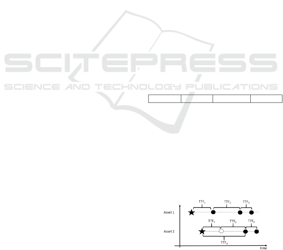
Survival data typically consists of times to failure

TTFs calculated from field data. For example

consider Figure 1. A fleet of 2 assets each in use since

the time marked by the star has experienced 6 failures

as shown by the dots in the graph. The delta between

the failures are the TTFs in this case there are 6 TTF

values. These values can be seen as the results of a

random variable f. The probability distribution

function behind f can be estimated using the TTFs.

The reliability function as described in Section 1 is

simply the inverse of f.

Figure 1: Collecting Times to Failure TTFs.

A plant’s CMMS is a good source of data for this

calculation. However, the data format is a little more

complex, which causes a series of data quality

problems. The subset of data relevant for our analysis

is approximated by the figure below.

Unlike in the data in Figure 1, the asset data does

not contain a list of relevant failure events. Instead,

both failure events and assets are associated with

functional locations to use the SAP term. A functional

location describes a function in the plant’s production

system “main feeder pump”. Assets are concrete

instances that can be installed at the locations “pump

A Data Quality Dashboard for CMMS Data

171

XYZ”. Over time, assets can move to different

locations as they are replaced with other assets,

repaired or overhauled and installed in other places.

Thus, the connection between asset and failure is only

an indirect one. As one can imagine, this is a key

source of data quality issues in a CMMS.

Figure 2: Key CMMS Data.

4 DATA QUALITY METRICS FOR

RELIABILITY DATA

We have already discussed data quality issues

affecting survival analysis in a previous paper (Gitzel,

2015). Thus, we have by now analysed six cases from

different contexts in order to identify the data quality

problems which affect a reliability calculation. The

latest case a customer’s CMMS system has led to the

discovery of new data quality problems, many of

which are unique to CMMS data.

In this section, we present an updated list of

metrics with a focus on those suitable for CMMS

data. For each metric, we describe the problem it

measures and the formula to calculate the metric. We

also describe the impact this problem has on a

survival analysis and propose ways how to address

this problem.

4.1 Sampling

4.1.1 Sampling Size

Problem: In order for a statistical analysis to be

relevant, we need a sample of an appropriate size. The

sample size needed depends on the standard deviation

of the population. The higher the standard deviation,

the more samples we need.

Metric:





  





where SEM is the Standard error of the mean and

MTBF is the mean. See (Gitzel, 2015) for more

details on this metric.

Impact: If sample size is too small, the sample does

not represent the full population properly. The

standard error of the mean estimates the possible

effect on the MTBF, other effects depend a lot on the

distribution function underlying the failure behaviour

if any.

Suggested Remedy: The obvious way to get reliable

survival statistics is to increase the sample size.

However, in many cases this would mean waiting for

more failures to occur which is not practical.

4.1.2 Observed Time Window

Problem. Observed time to failure TTF is the key

information needed to define a Reliability function.

In most cases TTF is the time between two failures,

except for the first failure, where it is the time since

start-up of the asset. This can lead to an interesting

problem in cases where the CMMS was installed after

plant start-up, because a lot of failure events will not

be recorded in the system.

Metric. The following metric calculates how much of

the plant lifetime is covered by the observed time

window recorded in the CMMS.















where 



is the total time of CMMS operation

and 



is the total time of plant operation. So, if the

plant is 40 years old and the CMMS was only

installed 20 years ago, the observed time window

would be 0.5.

Impact: The main problem of a small observed time

window is that we do not have access to the majority

of failure information. Moreover, if the difference

between plant lifetime and observed time window is

not taken into account, wrong TTFs will be included

in the list. In the figure below, stars represent the time

when an asset was started up, circles represent

failures. To the naïve observer it might seem that

there were no failures initially with failures showing

up only recently. However, this is an artefact of the

fact that failure recording started only with the

installation of the CMMS system the dotted line

parallel to the y axis. Thus, the long initial TTF is not

correct and the problem leads to an overestimation of

reliability.

ICORES 2018 - 7th International Conference on Operations Research and Enterprise Systems

172

Figure 3: Effect of Observed Time Window.

Suggested Remedy: The first TTF should be

removed and a left-censored time computed from the

difference between first failure and start-up be added.

This is a partial correction which works best if there

are enough “real” TTFs to compensate.

4.2 Consistency

Data is inconsistent if different names are used for the

same element. It is also inconsistent if quantitative

information uses different units inch vs. cm or scales

hours vs. days. Inconsistency often results from

merging different data sources. There are other

inconsistencies which are typically closely related to

a particular problem instance one of which is

described below.

4.2.1 Inconsistent Names

Problem: Important elements such as assets,

functional locations or related attributes use an

inconsistent notation. For example, an asset might be

correctly identified via the serial number but when a

particular failure report uses the inventory number of

the asset to refer to it.

Metric: A metric which can heuristically identify

values which do not adhere to the agreed naming

convention can use regular expressions to see which

values do not match the pattern suggested by the

convention e.g. serial number structures, see Fig 4.













where n is the number of all fields using a name

and 



is the number of name fields which match the

proscribed pattern.

Figure 4: Implementation of the Serial Number Consistency

Check.

Impact: Since we need to establish a link between

failure information and failures that were reported,

there needs to be a unique “key”. Otherwise, there

will be failures which cannot be assigned properly,

which a tremendous negative effect on the analysis

quality as has discussed in Section 5.2. In the case of

attribute names, we will not be able to properly build

subfleets for detailed analysis. A subfleet of all

“highly critical 3” assets will miss out all assets

labeled as “3” instead.

Suggested Remedy: Go through all identified non-

consistent values and try to change them to the correct

value. Inconsistencies can very often be resolved

through replacement rules.

4.2.2 Inconsistent Use of Functional

Locations

Problem. In a CMMS, functional locations might be

the only connection between the assets and the failure

events see Figure 2. In order for the analyst to be able

to connect a failure with an asset, the work order

reporting the failure must be connected to the right

asset. However, sometimes failures are linked to

locations higher in the hierarchy. So the best practice

might be that failures are attached to the leaves of the

functional location hierarchy e.g. pump AB.XYZ but

some failure reports might be attached to non-leave

nodes e.g. building AB instead.

Metric: 



as described above see Section 4.2.1.

Impact. Failures attached to the wrong functional

locations mean that these failures are not attributed to

the assets where they occurred. This means that there

are assets with higher TTFs which leads to an

overestimation of reliability.

Suggested Remedy: Sometimes further investigation

can help to find the right functional location but in

other cases the information about the proper leaf to

use might be lost.

4.3 Free-of-Error

There are two important categories of errors we can

detect with our metrics – syntactical errors and logical

errors. Logical errors include dangling keys e.g.

failure events referring to equipment which does not

exist, non-unique keys and illogical order of dates

such as failure date before manufacturing date.

4.3.1 Logical Errors - Dangling Keys

Problem: Sometimes elements in the data reference

each other. A typical problem is a failure event

referring to an asset or functional location which does

A Data Quality Dashboard for CMMS Data

173

not exist. Also, functional locations might refer to

assets which do not exist or vice versa.

Metric: A metric which measures the percentage of

working keys can be used discover the problem of

dangling keys.





  





, where d is the number of dangling

keys and n is the number of all keys.

Impact: Dangling keys mean that failure events

cannot be assigned to assets or that assets cannot be

assigned to functional locations. Both cases mean that

the reliability is overestimated.

Suggested Remedy: Very often, this problem is

caused by improper subfleet selection, i.e. we have

excluded elements which should still be in the list or

we have included items which should not be in the list

and now refer to other elements outside the scope.

Thus, this problem can often be resolved by looking

at the complete data set.

4.4 Completeness

Completeness is what most people seem to associate

with data quality. Completeness metrics essentially

depend on how much data is missing. In past papers,

we have detailed different completeness metrics,

however, we feel that these are the most important

ones.

4.4.1 Data Field Completeness

Problem: For a given column/data field, the value is

missing. A missing value can be empty or is

represented by text like “N/A”, “unknown”, “nan”

etc.

Metric: The column completeness metric tracks the

percentage of values in a particular data field which

are not empty.





  





, where e is the number of empty

fields and n is the number of all fields of this type.

Impact: The impact of empty fields varies with the

importance of a field. If the field is critical to the

calculation, this means that one asset cannot be used,

effectively reducing the sample size. If the field is

used for subfleet building it has the same effect once

sub-fleets are used. Substitution fields might not have

an impact as long as they value they can substitute is

of OK data quality.

Suggested Remedy: Sometimes missing values can

be filled in but there is a substantial risk that we will

use data generated based on our assumptions to

confirm those assumptions. We have made some

good experiences with scenario building (Gitzel,

2015).

4.4.2 Asset-function Location Mapping

Completeness

Problem: As shown in Figure 2, the connection

between functional locations and assets might be

needed to map failure events to assets. However, a

plant is not static and assets move to different

locations. Thus, if the asset-failure mapping is not

established at the time of the recording of the failure,

we need a table which documents at what time an

asset was found at what location. Sometimes, this

mapping has gaps.

Metric: The following metric tracks how many

failure events could not be assigned due to gaps in the

asset-location mapping.





  





, where e is the total number of

failure events and u is the number of failure events

which could not be assigned to an asset due to a gap

in the mapping.

Impact: The impact of unassigned events in

discussed in detail in Section 5.

Suggested Remedy: Restoring this information is

quite often not possible.

4.5 Plausibility

Often, data is not obviously wrong and thus marked

by the metrics in Section 3 but seems so improbable

that we at least have to consider the possibility that it

is wrong. What is plausible or not depends on the

context but there are some example metrics that are

useful in the context of CMMS data. All plausibility

metrics have the same basic format.





  





, where x is the name of the metric, v

is the number of elements that violate the plausibility

assumption and n is the total number of elements.

4.5.1 Double Tap

Problem: If two failures of the same asset occur one

after another in a very short time period a day or two,

the reason could be that the asset was not repaired

properly. However, more likely, there was a second

complaint about the same problem when no action

was taken the first time. In the second case, it might

make sense to remove one of the events. Otherwise,

ICORES 2018 - 7th International Conference on Operations Research and Enterprise Systems

174

the reliability will be severely underestimated. The

first case might stay in the data if we consider poor

repair to be a valid cause of failures or not if we count

this as one problem that took longer to fix.

Impact: The reliability will be severely

underestimated if there are many wrong double taps.

Suggested Remedy. If you feel a double tap is not

correct, remove the second or the first event. Given

the short time difference, your choice has no major

impact.

4.5.2 Failure after Replacement

Problem: According to the data, an asset was

replaced by another one without having failed.

However, the new asset fails almost immediately

afterwards. While such a scenario is certainly

possible, there is also the possibility that a

replacement was booked but the failure event still

belongs to the previous asset. In other words, the old

asset failed and was replaced with a new unit instead

of the old asset being replaced by a unit that failed

right away.

Impact: The reliability will be underestimated.

Suggested Remedy: Clarify each event or remove

the events. Only fix this problem automatically if you

are sure that assets are normally not replaced while

still working.

5 IMPACT OF DATA QUALITY

ISSUES

Data quality issues can have a series of effects. The

reliability curve can lead to systematic over- or

underestimation a “shift” to the right or left. In more

extreme cases, the shape is changed which means the

impact for a particular time t will differ. Also, a

changed shape can change the failure rate from

increasing to decreasing or vice versa. This has a

major impact on maintenance planning which cannot

be discussed in the context of this paper.

Examining all effects and understanding their

impact in order to scale our metrics is an effort

beyond the scope of this paper. However, there is a

large group of metrics that implies that a certain piece

of data cannot be used either because it is missing or

it is wrong. In these cases, either the sample size is

reduced or failure events need to be discarded. For

both cases, we can make a good estimate on whether

the extent of the data quality problem is still

acceptable or not.

5.1 The Effect of Problems Reducing

Sample Size

Both missing and wrong data can lead to a reduction

in the number of TTFs. For example, missing subfleet

information means that certain assets cannot be

included in the calculation. Syntactically wrong start

dates mean that we cannot calculate the TTFs for that

asset.

Typically, these problems are fixed by removing

the offending elements. This removed the problem as

such but reduces the sample size and thus the sample

size metric. For this reason, we need a good measure

as to what constitutes a good sample size.

The sample size metric as proposed in this paper,

estimates the typical percentage deviation introduced

by the small sample. Thus, a metric of 75% indicates

that the actual values might be  of the

calculated value. The percentage of deviation

acceptable depends on the use case. The analyst

should decide which relative deviation is still

acceptable for a particular type of analysis. If 



the deviation that is considered to be entirely

unproblematic and 



is a deviation that is still

acceptable, the following thresholds can be defined

for the metric



. These thresholds can be used for a

traffic-light design with states red (unacceptable),

green (acceptable), and yellow (insignificant).

Acceptable





 



Unacceptable





 



5.2 The Effect of Problems Leading to

Missing Failure Events

A number of data quality problems can lead to a

failure event not being assigned to an asset – either

because it cannot be assigned at all or because there

is reason to doubt the correctness of the assignment.

For example, due to the arrangement described in

Section 3, wrong or missing asset keys and wrong or

missing functional location keys mean that a given

event cannot be assigned to an asset see Section 4.4

for details.

Figure 5: Missing Failure Event.

A Data Quality Dashboard for CMMS Data

175

Furthermore, some events are lost due to a short

observation window see Section 4.1.3. Finally, failure

events which occur before the installation date and

other implausible events are most likely not correct

and should be evaluated Section 4.5.

The effect of a missing failure event is illustrated

in Figure 5. In the example, one of the events of asset

2 is missing (represented by the white circle). Thus,

instead of the correct times of failure TTF

and TTF

the wrong TTF

is added to the list. This means that

two correct TTFs are missing and one TTF that is far

too high is added by accident. Obviously, this leads

to an overestimation of reliability.

While this effect seems to suggest that unusually

high TTFs are suspicious, we cannot know which

ones are real and which ones are artefacts of missing

events. Based on our philosophy of identifying

problems and refraining from corrective actions

based on assumptions, we propose an impact

estimation heuristic. In order to identify thresholds

similar to the section above, we use a series of

simulations to determine possible data quality effects.

Due to the underlying assumptions see below, these

values should be taken as a rule of thumb and could

be refined in the future.

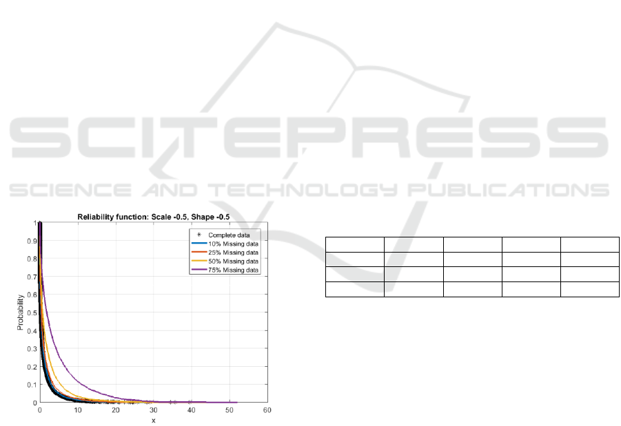
Our estimation is based on a series of simulations.

In each simulation we use a randomly generated

reliability curve and test the effect of missing events.

We use multiple percentages of randomly missing

events 10%, 25%, 50% and 75% and calculate an

alternative curve based on the reduced event set.

Figure 6: Typical Simulation Result.

Figure 6 shows a typical simulation result. The

black curve represents the correct reliability. The

coloured curves show the consecutive effect of

missing failure events. As expected, missing failure

events lead to an increasing overestimation of

reliability. For all our tested curves, the

overestimation is most pronounced in the middle of

the curve.

The simulation is based on a series of

assumptions. First, we need some random distribution

as a basis for our simulated curves. We follow

common practice and assume that all failure curves

follow a Weibull distribution. In order to cover a wide

range of possible scenarios, we use a series of

different shape and scale parameters selected to

represent different failure behaviours random,

increasing, decreasing, almost normally distributed

etc. Second, we assume that there is no wrong data

included in the calculation. Unrecognized wrong data

is a different issue which beyond the scope of the

metrics addressed here. Finally, for the sake of

simplicity, we assume that there will be no two

consecutive events missing. We argue that the effect

of will be more pronounced but not of a different

quality than what we see in our examples.

The overall results of the simulations are shown

in Table 1. For example, if 10% of the data is missing,

there will be a reliability overestimation anywhere

between 2.9 and 23.2 percentage points, depending

on curve shape. So, if we find a 25 percentage point

overestimation to be acceptable, we need a minimum

metric value of 75% taken from the 25% column,

since the metric is the inverse of the number of

missing events.

In this paper, we briefly outline our design

philosophy for a data quality dashboard. For a more

in-depth discussion see (Gitzel, 2015).

Table 1: Effect of missing events.

10%

25%

50%

75%

Max

23.2

23.5

47.3

71.5

Min

2.9

8.2

38.7

Average

7.9

15.0

30.9

53.0

6 CONCLUSIONS

Maintenance data collected in a production plant’s

information systems typically the CMMS is useful for

the analysis of asset reliability. However, various data

quality problems can impede this analysis. In this

paper we have presented a hierarchy of metrics

suitable for an assessment of the quality of CMMS

data. Based on several use cases, we have identified

relevant metrics and proposed criteria to structure

them. Finally, we have proposed heuristics needed to

decide whether a metric result is good or bad.

In our opinion, the sensitivity of survival analysis

to data quality issues is quite severe – a finding we

did not expect. To us this implies that in order for

ICORES 2018 - 7th International Conference on Operations Research and Enterprise Systems

176

survival analysis to work, we need to either come up

with good measures to ensure data quality or to find

algorithms which can correct the problems.

However, in the light of recent developments such as

Industrie 4.0 and Industrial Internet, maybe the

alternative is to primarily rely on condition

monitoring data. Of course, this means that there will

be other data quality issues to be addressed and future

research is required.

REFERENCES

R. G. Miller 1997. Survival analysis, John Wiley & Sons.

J. Antoni, J.; R. B. Randall 2006. The spectral kurtosis.

Application to the vibratory surveillance and

diagnostics of rotating machines. In Mechanical

Systems and Signal Processing.

R. Gitzel, S. Turring and S. Maczey 2015. A Data Quality

Dashboard for Reliability Data. In 2015 IEEE 17th

Conference on Business Informatics, Lisbon.

R. Gitzel 2016. Data Quality in Time Series Data - An

Experience Report. In. Proceedings of CBI 2016

Industrial Track, http.//ceur-ws.org/Vol-

1753/paper5.pdf.

IEEE 2007. IEEE Standard 493 - IEEE Recommended

Practice for the Design of Reliable Industrial and

Commercial Power Systems.

S. Kunttu, J. Kiiveri 2012. Take Advantage of

Dependability Data, maintworld, 3/2012.

J.W. Hines, A. Usynin 2008. Current Computational Trends

in Equipment Prognostics. In International Journal of

Computational Intelligence Systems.

M. Salgado, W. M. Caminhas W.M; B. R. Menezes 2008.

Computational Intelligence in Reliability and

Maintainability Engineering. In. Annual Reliability and

Maintainability Symposium - RAMS 2008.

S. Wu, A. Akbarov 2012. Forecasting warranty claims for

recently launched products. In Reliability Engineering

& System Safety.

R. Vadlamani 2007. Modified Great Deluge Algorithm

versus Other Metaheuristics in Reliability

Optimization, Computational Intelligence in Reliability

Engineering, Studies in Computational Intelligence.

R. Gitzel, C. Stich 2011. Reliability-Based Cost Prediction

and Investment Decisions in Maintenance – An

Industry Case Study, In. Proceedings of MIMAR,

Cambridge, UK.

Bertino, E.; Maurino, A.; Scannapieco, Monica 2010. Guest

Editors’ Introduction. Data Quality in the Internet Era.

In Internet Computing, IEEE.

D.P. Ballou et al. 1997. “Modeling Information

Manufacturing Systems to Determine Information

Product Quality”, Management Science.

Borek, A.; Parlikad, A. K.; Webb, J.; Woodall, P. 2014.

Total information risk management – maximizing the

value of data and information assets.

Bertino, E.; Maurino, A.; Scannapieco, M. 2010. Guest

Editors’ Introduction. Data Quality in the Internet Era.

In Internet Computing, IEEE.

Becker, D.; McMullen W.; Hetherington-Young K. 2007.

A flexible and generic data quality metamodel. In

Proceedings of International Conference on

Information Quality.

Montgomery, N.; Hodkiewicz, M. 2014. Data Fitness for

Purpose. In. Proceedings of the MIMAR Conference.

Delonga, M. Zuverlässigkeitsmanagementsystem auf Basis

von Felddaten. Universität Stuttgart.

Bendell, T. 1988. An overview of collection, analysis, and

application of reliability data in the process industries.

In Reliability, IEEE Transactions.

Redman, T.C., ed. 1996. Data Quality for the Information

Age.

Leo L. Pipino, Yang W. Lee, Richard Y. Wang 2002. “Data

Quality Assessment”, Communications of the ACM.

Bovee, M.; Srivastava, R. P.; Mak, B. 2003. A Conceptual

Framework and Belief-function Approach to Assessing

Overall Information Quality. In. International Journal

of Intelligent Systems.

Peter Benson 2008. ISO 8000 the International Standard for

Data Quality, MIT Information Quality Industry

Symposium.

Xiaojuan, Ban; Shurong, Ning; Zhaolin, Xu; Peng, Cheng

2008. Novel method for the evaluation of data quality

based on fuzzy control. In Journal of Systems

Engineering and Electronics.

Damerau, Fred J. 1964. A technique for computer detection

and correction of spelling errors. In Communications of

the ACM.

Levenshtein, Vladimir I. 1966. Binary codes capable of

correcting deletions, insertions, and reversals, In Soviet

Physics.

Bard, Gregory V. 2007. Spelling-error tolerant, order-

independent pass-phrases via the Damerau–

Levenshtein string-edit distance metric, In Proceedings

of the Fifth Australasian Symposium on ACSW.

Wu, Shaomin 2013. A review on coarse warranty data and

analysis, In. Reliability Engineering & System Safety.

Hu, X. Joan, Lawless, Jerald F. 1996. Estimation of rate and

mean functions from truncated recurrent event data. In

Journal of the American Statistical Association.

Gitzel, R. 2014. Industrial Services Analytics. Presentation

at the 1. GOR Analytics Tagung.

A Data Quality Dashboard for CMMS Data

177