
Image Features in Space
Evaluation of Feature Algorithms for Motion Estimation in Space Scenarios
Marc Steven Kr¨amer, Simon Hardt and Klaus-Dieter Kuhnert
Institute of Realtime-Learning Systems, University of Siegen, Hoelderlinstr. 3, 57076 Siegen, Germany
Keywords:
Visual Odometry, Motion Estimation, Space Robotics, SIFT, SURF, BRIEF, ORB, KAZE, AKAZE, BRISK.
Abstract:
Image features are used in many computer vision applications. One important field of use is the visual naviga-
tion. The localization of robots can be done with the help of visual odometry. To detect its surrounding, a robot
is typically equipped with different environment sensors like cameras or lidar. For such a multi sensor system
the exact pose of each sensor is very important. To test, monitor and correct these calibration parameters, the
ego-motion can be calculated separately by each sensor and compared. In this study we evaluate SIFT, SURF,
ORB, AKAZE, BRISK, BRIEF and KAZE operator for visual odometry in a space scenario. Since there was
no suitable space test data available, we have generated our own.
1 INTRODUCTION
Over the years a variety of methods and algorithms
for the detection and extraction of image features have
been developed in digital image processing and com-
puter vision. Typical application are object track-
ing, image retrieval, panorama stitching or camera
pose estimation. An important and common usage
for accurate localization, especially in the field of mo-
bile robotics, is the visual odometry (Scaramuzza and
Fraundorfer, 2011). This is the process of ego-motion
and pose estimation for a mobile robot by analysing
the images of an attached camera.
To detect the surrounding environment, a robot
can be equipped with several sensors. These are for
example (stereo) cameras, lidar, ultrasonic or radar.
All these sensor data can be combined into a consis-
tent environment model. For this sensor registration
and fusion process, the exact positions and orienta-
tions (pose) of all sensors are extremely important.
These data is normally obtained during a calibration
of the whole system. A way to check and monitor
these parameters is based on the robots ego-motion,
which is estimated separately from the sensing data
of the different sensors. A comparison with a ground
truth, in our case a high precise fibre optical inertial
measurement unit (IMU), allows to verify the proper
calibration and offers in a second step the possibil-
ity to correct it. During the motion estimation (visual
odometry) with a camera, image features are a cen-
tral aspect for calculating the pixel shifts of successive
images (Fraundorfer and Scaramuzza, 2012).
The evaluation which is published in this paper is
part of a bigger project called AVIRO, where a sensor
fusion system for space robotic is developed. There-
fore, we tested different feature algorithms for the us-
age in a space scenario.
In the literature a variety of evaluations for feature
algorithms have been published. Most of them anal-
yse different feature algorithms with a dataset pro-
posed by (Mikolajczyk and Schmid, 2003) and which
consists of images with real geometric and photo-
metric transformations. These are rotation, scale
changes, viewpoint changes, image blur or illumina-
tion changes. (Canclini et al., 2013) evaluated the
processing time, repeatability and matching accuracy
for image retrieval task. For object tracking in a
video (Sebe et al., 2002) evaluatedSIFT, SURF, ORB,
BRISK, FREAK and BRIEF. (Miksik and Mikola-
jczyk, 2012) focused in an evaluation for fast feature
matching on the speed of the matching process. After
a summary of all papers it can be said, that the ideal
operator depends on the application. This also results
from (Is¸ık, 2014).
Evaluations of features for visual odometry have
been made for typical road scenes in (Qu et al., 2016).
Also (Chien et al., 2016) investigated different feature
algorithms for visual odometry on the street and sug-
gested SURF as the best algorithm. The performance
of SIFT and SURF in case of a stereo camera was
evaluated by (Jiang et al., 2013) on a road scene in
an urban environment and by (Benseddik et al., 2014)
with a robot inside a building.
Other publications evaluated the operators with a
300
Krämer, M., Hardt, S. and Kuhnert, K-D.
Image Features in Space - Evaluation of Feature Algorithms for Motion Estimation in Space Scenarios.
DOI: 10.5220/0006555303000308
In Proceedings of the 7th International Conference on Pattern Recognition Applications and Methods (ICPRAM 2018), pages 300-308
ISBN: 978-989-758-276-9
Copyright © 2018 by SCITEPRESS – Science and Technology Publications, Lda. All rights reserved
data set of plant species (Kazerouni et al., 2015) or
UAV images (Yumin et al., 2016). Especially for the
field of space robotics, more precisely a planetary sce-
nario, (Shaw et al., 2013) tested the BRIEF algorithm
for a robust visual odometry in a sand quarry in Ox-
fordshireUK. (Maimoneet al., 2007) concluded in his
publications about visual odometry on mars rovers,
that for a robust technology, the runtime of the algo-
rithms is the bottleneck.
This paper is organized as follows: In section 2 we
describe our test data set. The recording of a real and
generation of a virtually simulated scene. After this in
section 3, the method of comparison and evaluation is
presented before we discuss the results in section 4.
Finally, the paper is concluded in section 5.
2 GENERATION OF
TESTSCENES
Research publications on feature operators are usu-
ally a comparison which is geared to the needs of the
specific application. Algorithms were applied to real
or virtual test scenes and compared to ground truth
data. This involves mainly the simple retrieval of ob-
jects or object points in two or more different images.
Here objects are everyday objects, such as a boats
(Benseddik et al., 2014), graffiti (Miksik and Mikola-
jczyk, 2012), trees (Is¸ık, 2014) or hands (Sebe et al.,
2002). In order to find suitable operators e.g. for plant
recognition, a test database with many photos under
varying settings (exposure time, camera angle, lens,
digital resolution and other parameters) is created.
There are own test scenes for more specific applica-
tion areas. In the automobile sector a road scene was
recorded by a camera and the ground truth data was
extracted from an intertial measurement unit (Geiger
et al., 2013). In addition to the feature algorithms, the
quality of a visual odometry can be measured at the
same time.
The special application in the project AVIRO is
the space robotic. Thus suitable test databases were
also created for the evaluation of the feature algo-
rithms. By using features, pose changes of a robot in
(outer) space were estimated. It is therefore obvious
to generate test data for this special purpose.
So we created a simplified scenario to test the al-
gorithms for this visual odometry application. A cam-
era rotates around its own axis. During the rotation
the exact rotation angle is measured and recorded par-
allel to the video. With this relatively simple method,
several scenes were generated in a simulated virtual
and a real environment. All image data has been saved
as raw images without any compression.
2.1 Real Enviroment
AVIRO is developed in the offices and laboratories of
the University of Siegen. Therefore, a part of the test
database consists of scenes in this environment. For
the recordings the mono camera UI-5360CP from ids
imaging has been used. Figure 1 shows the used test
setup and table 1 provides information about the cam-
era.
Table 1: Technical data of the mono camera UI-5360CP
from ids imaging.
Sensor CMOS 2/3”
Resolution 2048x1088
Framerate 36Hz
A carrier board is mounted on a photo tripod on
which the camera and a fiber gyroscope are installed.
Above, there are additional electrical circuits which
stably produce the complex voltage supply for the
gyro system. The fiber gyro is the µFORS-1 model
from Northrop Grumman Litef which is also used for
aircraft navigation or rocket control. Technical data
can be found in table 2.
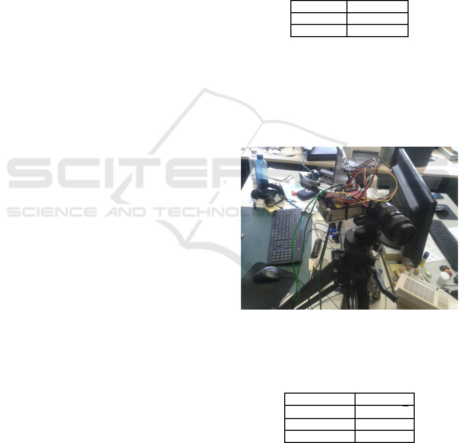
Figure 1: Test setup for recording data in a real environ-
ment. The photo shows the test setup for recording test
data. The used monocamera UI-5360CP is mounted on a
tripod together with a high-precision fiber gyro. During the
recordings the setup was rotated around the vertical axis.
Table 2: Technical Data of the fiber gyro µFORS-1.
Rate Bias ≤ 1
◦
/h
Random Walk ≤ 0,1
◦
/
√
h
Gyro Range ±1000
◦
/s
Max data rate 8kHz
During a rotation of the tripod a video stream with
a framerate of 30Hz is created by the camera. Simul-
taneously, the fiber gyro records the rotation at 1 kHz.
Image Features in Space - Evaluation of Feature Algorithms for Motion Estimation in Space Scenarios
301
The camera stands directly on the vertical axis and ro-
tates without a translatory effect. Since this is a cam-
era of industrial quality, a consistent timing behaviour
can be assumed and the triggering time of each frame
is known. This results in a test dataset in which an
exact rotational position of the tripod can be assigned
to each image. This rotation angle is the ground truth
value for later evaluations.
Several test records have been created in this con-
figuration. Figure 2 shows an example of four images
of the generated video sequences. It is a typical office
environment, as it also prevails with most of all other
tests. However, this kind of test is more suitable for
mobile ground robotsand less for the use on satellites.
Therefore, further data records for the feature evalu-
ation were generated which are described in the next
section.
Figure 2: Example images of a test scene in real environ-
ment.
2.2 Simulated Environment
The planned operational environment of the finished
AVIRO system is in space. This differs significantly
from the created test data described in the previous
section. As no suitable data was available for this test,
it had to be created. In order to obtain realistic test
data it was decided to simulate a space scene virtually
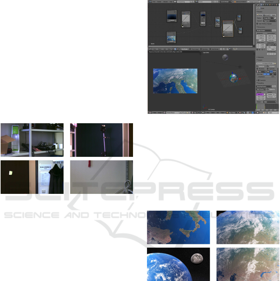
on the computer. As a tool the open source 3D ren-
dering software Blender was used. An existing and
Creative Commons licensed space scene by Adriano
Oliveira (Oliveira, 2014) was extended with a higher
resolution texture of the Earth’s surface (see figure 3).
Figure 4 shows some rendered example images. A to-
tal of five test recordingswere made. For this purpose,
the camera was positioned in five different locations
in the virtual space environment and rotated with a
fixed angle around an axis by an animation. It was
noticed that the camera is aimed at different objects
of the scene. Thus, a mixture of images of the earth’s
surface and the further space or other planets (moon)
could be generated - a simulation of conceivable
states of a satellite.
The Blender software offers the possibility to
Figure 3: Generation of the simulated virtual scene with
Blender.
specify the camera parameters with which the virtual
scene is drawn. As a result, focal length, resolution
and chip size could be adapted to the data of the real
camera (ids imaging UI-5360CP). The ground truth
data are available directly in the program, since the
camera position or, more correctly, its orientation, is
known. Here, as in the first real scene, the camera
was rotated virtually about an axis. Thus, datasets
with image and angle pairs have been created which
are available for later tests.
Figure 4: Sample images of a test scene in a simulated vir-
tual environment.
2.2.1 Simulated Sensor Noise
The second dataset contains images generated by the
Blender software. Colors in the space scene are ideal
mapped (taking into account the illumination condi-
tions) on the resulting images. However, this does not
reflect the indeed real behaviour of a video camera.
The sensor noise which causes a falsification of the
color values is as an important point not considered.
In order to include the influence of this effect, noise
was artificially added to the image data of the simu-
lated scenes in a further step. This takes place in two
ICPRAM 2018 - 7th International Conference on Pattern Recognition Applications and Methods
302
stages.
The dataset contains RGB images with a color
depth of 8 bits. First, the image matrix is converted
from RGB to the HSV color model. In the HSV
color space, a uniform, random value between −15
and +15 is added to the brightness component (V).
This simulates variations in the exposure time. After
re- converting to RGB a random value between −20
and +20 is added to each component. This produces
the sensor noise in reality. For the calculation opera-
tions overflow or underflowof the 8-bit numeric space
is handled. For values < 0 the value is set to 0 or if
> 255 to 255.
3 COMPARISON OF THE
ALGORITHMS
A large number of different algorithms for feature de-
tection and description have been developed so far.
In addition it is an active research area in which new
methods are continually developed. Furthermore,
each of the algorithms can be parameterized. This
creates a lot of possible combinations and makes it
harder to choose from these the best working solution
for our project. In order to make this decision, some
test datasets were generated which have already been
described in the last sections.
3.1 Method
Each of the generated test dataset contains a sequence
of pairs consisting an image and the corresponding
camera angle. The evaluation of feature algorithms is
now based on the principle that the camera rotation
between two consecutive images is calculated (pixel
shift). This value is compared with the Ground Truth,
which is contained in the test datasets. The single
steps of this procedure are described in more detail
below. Algorithm 1 also shows the method in a com-
pact way.
The evaluation has been done on a Desktop Com-
puter with Ubuntu 14.04 LTS. The system was an
Intel(R) Core(TM) i7-4930K CPU with 3.40GHz,
12MB Cache and 64 GB RAM. The opencv version
was 3.1.0 with the related opencv
contribute package
for the non free feature algorithms and compiled with
gcc version 4.8.4.
Load Image and Rectify. The first image is loaded.
With help of the camera parameters, which were
determined in the sensor calibration, distortions
caused by the lens can be corrected. This is not
necessary in the simulated scene and the virtual
camera.
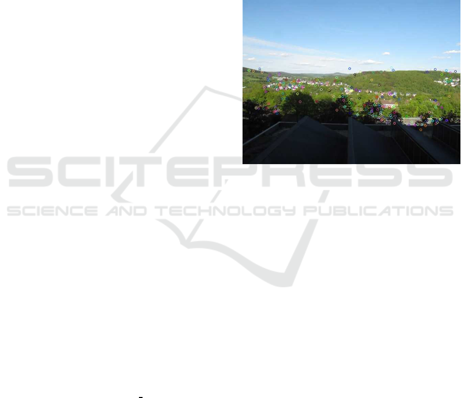
Find Keypoints. In the image keypoints have to be
found which can be easily found again the next
consecutive image. Each feature generation al-
gorithm basically consists of two parts: the de-
tector and the descriptor. In the first step the de-
tector is used to search for keypoints which are
very different from their surroundings. In simpli-
fied terms these can be locations where for exam-
ple a bright/dark transition is located. Figure 5
shows the SIFT detector applied to a sample im-
age. Marked points are represented by small cir-
cles.
Figure 5: SIFT detector applied to a sample image. The
figure illustrates the detector of the Scale Invariant Feature
Transform (SIFT) algorithm. In the picture keypoints which
are suitable for feature operations are drawn.
Specification of the Points by Descriptors. The
previously found points are now represented
by descriptors. A descriptor is a vector with
numbers. These are attributes that characterize
the point. For this purpose the surrounding of
the point, i.e. the neighboring pixels, are also
included. More detailed information, as an
example for the descriptor of the SIFT procedure,
can be found in (Lowe, 2004).
Load Next Image. The next image of the test dataset
is loaded and rectified. Here the camera has been
rotated by a certain angle. As with the previously
processed image, keypoints are searched and de-
scribed by descriptor vectors.
Comparison of Keypoints. The comparison be-
tween the feature vectors from the first and the
second image (matching) follows. Figure 6 shows
this procedure using an image of the real scene.
The pixels of the feature vectors which have been
identified as equal by the matching process are
connected with lines. It can be seen that not all
lines have the same orientation.
Image Features in Space - Evaluation of Feature Algorithms for Motion Estimation in Space Scenarios
303
The difference between the x- and y-components
of the image points of each matched point-pair is
the displacement. In figure 7 the distribution of
these is plotted. The majority of the points ac-
cumulate in a cluster, as can be seen in the his-
tograms to the right and below. Also, there are
some outliers that reflect the wrong lines in the
picture.
Estimate the Camera Rotation. The keypoint
matching process yields a set of keypoint pairs.
In a first step a filter is applied to filter out some
outliers in these data. The comparison of feature
vectors provides as a result a quality value which
indicates how good the vectors fit together. Based
on these values the best fifty pairs are extracted.
This is shown for the previous example in bottom
image of figure 6. Now the connected lines of the
keypoints have approximately the same length
and orientation. This can be seen in plot 8.
The range in which the points are located is sig-
nificantly reduced comparedto the previousdistri-
bution from 7. For the calculation of the camera
rotation we use the median of these values. This is
also shown in the whiskey boxplots on the sides.
Since the camera has only been rotated around a
single axis, the rotation of the camera can now be
calculated by means of the pixel shift (in this ex-
ample in the x-direction). The necessary camera
parameters, such as the aperture angle and focal
length, are known by the camera calibration. The
pixel shift in y-direction is 2.45 pixels which is
equivalent to 0.029
◦
. In the x-direction, there are
106.94 pixels and 1.28
◦
respectively. The low y-
deviation can be explained by sensor noise, back-
lash in the camera mounting or calibration errors.
4 EXPERIMENTAL RESULTS
Comparative tests were performed with seven fea-
ture algorithms. These are named after their ab-
breviations. Following the used algorithms are
listed. For a detailed description of the individ-
ual methods we refer to the literature.
SIFT. Scale-Invariant Feature Transform (Lowe,
2004)
SURF. Speeded Up Robust Features (Bay et al.,
2006)
BRIEF. Binary Robust Independent Elementary
Features (Calonder et al., 2010)
ORB. Oriented FAST and Rotated BRIEF
(Rublee et al., 2011)
Algorithm 1: Evaluation of feature algorithms.
Input: Data set with image and angle pairs
T = (I
0
,α
0
),(I
1
,α
1
),...,(I
n
,α
n
)
Output: Quality value s
f
of the feature
algorithm f
1 s
f
= 0
descriptors
prev
=f.describe(f.detect(I
0
));
2 for i = 1 to size(T) do
3 descriptors
curr
=f.describe(f.detect(I
i
));
4 pairs=Best
50
(match(descriptors
prev
,
descriptors
curr
));
5 calculate pixel shift ∆x with pairs;
6 calculate rotation angle β with ∆x;
7 s
f
=s
f
+ |β −α
i
—; //sum up error
8 descriptors
prev
= descriptors
curr
;
KAZE. KAZE-Features (Alcantarilla et al.,
2012)
AKAZE. Accelerated-KAZE Features (Pablo
Alcantarilla (Georgia Institute of Technolog),
2013)
BRISK. Binary Robust Invariant Scalable Key-
points (Leutenegger et al., 2011)
The previously generated test database is divided into
a simulated and a real environment. Therefore, the
results of the comparison are also considered sepa-
rately. Figure 9 shows consecutive images of both en-
vironments. Detected keypoints and their determined
agreement in the second picture are drawn. Totally
there are two datasets (T
R
0
, T
R
1
) in real and five (T
S
0
,
T
S
4
) in the simulated environment.
For the first test T
R
0
, the measurement setup (see
image 1) has been rotated by 90
◦
in a time of about 20
seconds. The reference value (Ground Truth) of this
dataset was determined with a high-precision fiber
gyro. In the measurement results the calculated angle
from all feature algorithms deviates. After a rotation
of 87.76
◦
(reference value) the calculated values of
the algorithms are between 90.46
◦
and 91.16
◦
. The
difference between the optical methods is therefore
only 0.7
◦
. More important is the question why there
is a systematic error between all calculated values and
the reference. When examining this behavior and the
underlying calculation steps, attention is immediately
drawn to the sensor calibration of the camera.
Camera calibration is a mathematical minimiza-
tion which never provides a hundred-percent cor-
rect solution. It has been done with the checker-
board method (see (Tsai, 1986)). An opening angle
of 0.01196655
◦
per pixel in x-direction can be fol-
lowed by the camera calibration. A 90 degree rota-
tion causes a displacement of 7590 pixels (BRISK
method). Smaller deviations in the aperture angle
ICPRAM 2018 - 7th International Conference on Pattern Recognition Applications and Methods
304
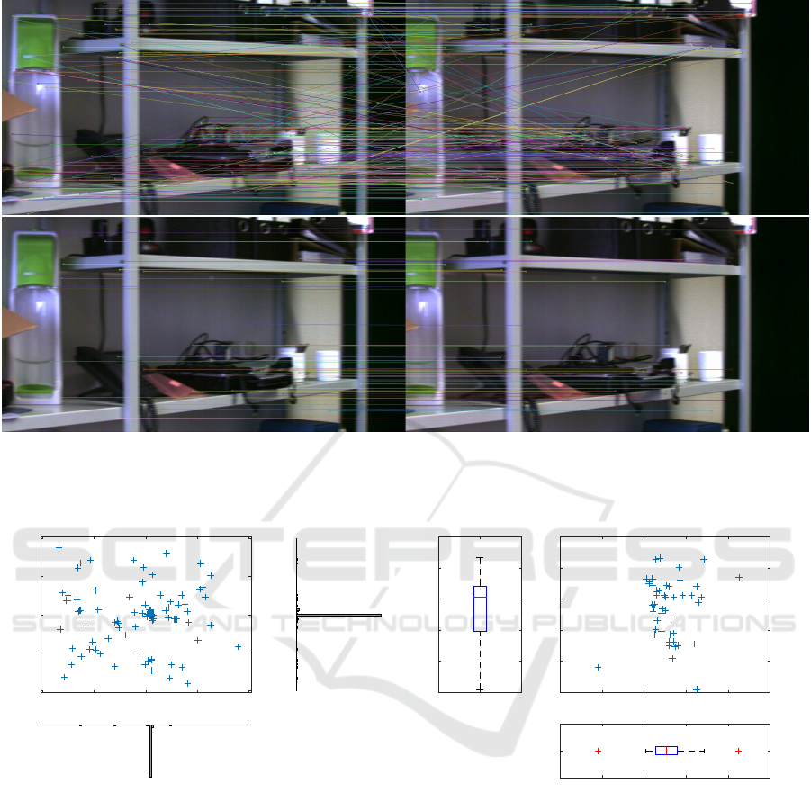
Figure 6: Finding feature point-pairs. Shown are two camera images in which the camera was rotated around an angle of a
few degrees. Keypoints detected by a feature detector are shown in the images. The lines connect points identified as being
the same in a matching process. On the top image 280 point pairs are shown. In the version below the best matching fifty
pairs were extracted.
x
-2000 -1000 0 1000 2000
y
-1000
-500
0
500
1000
Figure 7: Feature Point Matching. The plot shows the dis-
placement of the individual pairs in the x- and y-directions
of the matching process in figure 6 on the top. On the sides
are histograms. The total of points is 280.
therefore strongly influence the final result. In ad-
dition the correction of the lens distortion (rectificta-
tion) is added which has also been determined during
the camera calibration and can also falsify the values.
With further tests and new calibrations no signif-
icant improvement could be achieved. The key find-
ing from these results is that the angular changes can
only be viewed at shorter intervals. This is can also
be seen in figure 10. This graph shows the error of
the calculated angle. At the top it is summed up and
on the bottom shown stepwise. The plots indicate
the error in degrees. The summed error in pixels is
x
95 100 105 110 115 120
y
-5
-4
-3
-2
-1
0
Figure 8: Filteredfeature points. The boxplot shows the dis-
tribution of the 50 best feature point of the data. The median
is symbolized by the red line and the blue box correspond
to the 0.25 or 0.75 quantiles. The length of the whiskers is
1.5 times the interquartile distance. Outliers are represented
by red crosses. The displacement along the x-axis reflects
the rotation of the camera. The y-shift would have to be 0.
However it is shifted by sensor noise or calibration errors.
230.51px where the average error per step is 2.15px.
This equals 0.02
◦
. In order to achieve a better com-
parison with the simulated test data it is important to
note that only every fifth images was taken from the
30hz video stream to test the real scenes. This step
provides a rotation of about one degree per image.
Thus the average error per step is below three percent.
A summary of the individual in T
R
0
errors is pro-
Image Features in Space - Evaluation of Feature Algorithms for Motion Estimation in Space Scenarios
305
Figure 9: Feature Matching in both environment of the test
dataset. The illustrations show in each case two images of
the test dataset in the real and simulated environment. The
SIFT algorithm was applied to the images. The radius spec-
ifies the size of the keypoint. In addition the orientation is
indicated. Corresponding keypoints are connected with a
line.
0 10 20 30 40 50 60 70 80 90 100
step
-2
0
2
4
angle (°)
0 10 20 30 40 50 60 70 80 90 100
step
-0.5
0
0.5
angle (°)
SIFT
SURF
ORB
AKAZE
BRISK
BRIEF
KAZE
Figure 10: Errors of all feature algorithms in T
R
0
. Cumu-
lated error on the top, stepwise below.
SIFT SURF ORB AKAZE BRISK BRIEF KAZE
-0.5
-0.4
-0.3
-0.2
-0.1
0
0.1
0.2
0.3
0.4
0.5
angle error (°)
Figure 11: Boxplot of errors in T
R
0
. A green zero line is
indicated for better clarity.
vided by the boxplot in figure 11. Here the errors are
shown for each feature algorithm. It is easy to see that
there are no big differences between the algorithms in
this test scene.
In figure 12 the error values of both real scenes
T
R
0
and T
R
1
are summarized. T
R
0
is a left rotation
around 90 degrees. Scene T
R
1
is the same rotation the
other way (right) back to the initial point. This fact
explains the displacement of the median to the zero
point. Nevertheless there is no major difference be-
SIFT SURF ORB AKAZE BRISK BRIEF KAZE
angle error (°)
-0.4
-0.3
-0.2
-0.1
0
0.1
0.2
0.3
0.4
0.5
Figure 12: Boxplot of errors in T
R
0
and T
R
1
. A green zero
line is indicated for better clarity.
0 10 20 30 40 50 60 70 80 90
step
-0.5
0
0.5
1
1.5
angle error(°)
0 10 20 30 40 50 60 70 80 90
Schritt
-0.02
0
0.02
0.04
angle error (°)
SIFT
SURF
ORB
AKAZE
BRISK
BRIEF
KAZE
Figure 13: Errors of all feature algorithms in T
S
0
. Cumu-
lated error on the top, stepwise below.
tween the algorithms since the calibration effects (e.g.
lens distortion) are much stronger than the differences
of the operators.
The second tested dataset consisted of six simu-
lated scenes. In contrast to the previous real scenes
no camera calibration has to be generated here. These
parameters could be specified during the simulation
and were applied when the images were created. Fig-
ure 13 shows the summed and single errors for T
S
0
. In
the simulated scene the difference between the algo-
rithms is clearly visible. This also shows the boxplot
of this data in figure 14.
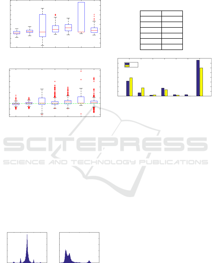
A summary of all simulated scenes T
S
i
= T
S
0
..T
S
5
shows figure 15. It can be seen that the feature algo-
rithms SIFT and SURF have the best quality. In order
to obtain a meaningful comparison value from the re-
sults of the tested feature algorithms, the error sum
was formed in each case. This is shown in table 3
for each algorithm and provides SIFT method as the
winner.
The previous tests pointed out SIFT as the most
appropriate feature algorithm. In addition to the an-
gular errors the average runtimes were also measured
during the tests. The diagram in 17 shows this. The
runtimes of the feature detectors and extractors were
determined separately. The graph shows that the cal-
culation time of the algorithms varies widely. While
the total duration of BRIEF is less than 0.1 seconds
ICPRAM 2018 - 7th International Conference on Pattern Recognition Applications and Methods
306
SIFT SURF ORB AKAZE BRISK BRIEF KAZE
-0.01
-0.005
0
0.005
0.01
0.015
0.02
0.025
0.03
0.035
angle error (°)
Figure 14: Boxplot of errors in T
S
0
. A green zero line is
indicated for better clarity.
SIFT SURF ORB AKAZE BRISK BRIEF KAZE
angle error (°)
-0.04
-0.02
0
0.02
0.04
0.06
0.08
0.1
0.12
Figure 15: Boxplot of errors in T
S
i
. A green zero line is
indicated for better clarity.
(0.07s detector + 0.004 s extractor), KAZE needs an
average of 2.7 seconds (1.5 s + 1.2 s) more than 30
times of the BRIEF time. The SIFT algorithm also
has a high runtime of 1.4 seconds (0.64s + 0.78s.
Another interesting evaluation of the test scenes is
the distribution of the determined pixel shift. This is
shown in figure 16. The data is based on the results of
three scenes in the simulated environment and a total
of 300 images (with 50 point pairs each) in which the
camera was rotated around the y-axis. The left plot
shows the shift on the X axis. Since this has not been
affected by the rotation the value 0px is expected. To
the right is the distribution of the y-shift. Their opti-
mal (Ground Truth) value is 15.9px. As opposed to
the normal distribution of the x-shift, this distribution
is multimodal. A possible explanation are rounding
during the scene rendering in Blender.
-3 -2 -1 0 1 2 3
x-shift (px)
0
100
200
300
400
500
count
15.5 16 16.5 17 17.5
y-shift(px)
0
100
200
300
400
500
Figure 16: Distribution of the shift in a simulated scene.
Table 3: Root Mean Square (RMS) of the feature algorithms
in the simulated scene.
SIFT 2.4359
SURF 2.7549
ORB 10.3270
AKAZE 5.3275
BRISK 5.9131
BRIEF 9.3461
KAZE 5.9881
SIFT SURF ORB AKAZE BRISK BRIEF KAZE
0
0.2
0.4
0.6
0.8
1
1.2
1.4
1.6
time (s)
Detector
Extractor
Figure 17: Runtimes of the feature algorithms.
5 CONCLUSIONS
In this paper we evaluated different feature algorithms
for the usage in a space scenario. These are namely
SIFT, SURF, ORB, AKAZE, BRISK, BRIEF and
KAZE. Since there was no test data for the special ap-
plication of space robotic available, two scenes were
created. One in our offices and the other in a virtually
generated space scene, which is a more realistic op-
erational environment. The feature algorithms have
been evaluated by a rotation of the camera. By com-
paring the estimated and ground truth angle a rank-
ing was made. In our case the scale invariant feature
transform (SIFT) algorithm provided the best results.
Since visual odometry has to be real-time capabil-
ity, we also evaluated the runtimes. The SIFT algo-
rithm has a high runtime and is thus not realizable in
realtime. Even with a smaller framerate. For this rea-
son the implementation of SIFT in our space project
AVIRO is carried out in hardware.
REFERENCES
Alcantarilla, P. F., Bartoli, A., and Davison, A. J. (2012).
Computer Vision – ECCV 2012: 12th European Con-
ference on Computer Vision, Florence, Italy, October
7-13, 2012, Proceedings, Part VI, chapter KAZE Fea-
tures, pages 214–227. Springer Berlin Heidelberg,
Berlin, Heidelberg.
Bay, H., Tuytelaars, T., and Gool, L. V. (2006). Surf:
Speeded up robust features. In Proceedings of the
ninth European Conference on Computer Vision.
Image Features in Space - Evaluation of Feature Algorithms for Motion Estimation in Space Scenarios
307

Benseddik, H. E., Djekoune, O., and Belhocine, M. (2014).
Sift and surf performance evaluation for mobile robot-
monocular visual odometry. Journal of Image and
Graphics, 2(1).
Calonder, M., Lepetit, V., Strecha, C., and Fua, P. (2010).
Computer Vision – ECCV 2010: 11th European
Conference on Computer Vision, Heraklion, Crete,
Greece, September 5-11, 2010, Proceedings, Part IV,
chapter BRIEF: Binary Robust Independent Elemen-
tary Features, pages 778–792. Springer Berlin Heidel-
berg, Berlin, Heidelberg.
Canclini, A., Cesana, M., Redondi, A., Tagliasacchi, M.,
Ascenso, J., and Cilla, R. (2013). Evaluation of low-
complexity visual feature detectors and descriptors. In
2013 18th International Conference on Digital Signal
Processing (DSP), pages 1–7.
Chien, H. J., Chuang, C. C., Chen, C. Y., and Klette, R.
(2016). When to use what feature? sift, surf, orb,
or a-kaze features for monocular visual odometry. In
2016 International Conference on Image and Vision
Computing New Zealand (IVCNZ), pages 1–6.
Fraundorfer, F. and Scaramuzza, D. (2012). Visual odom-
etry: Part ii: Matching, robustness, optimization, and
applications. IEEE Robotics & Automation Magazine,
19(2):78–90.
Geiger, A., Lenz, P., Stiller, C., and Urtasun, R. (2013).
Vision meets robotics: The kitti dataset. International
Journal of Robotics Research (IJRR).
Is¸ık, S¸. (2014). A comparative evaluation of well-known
feature detectors and descriptors. International Jour-
nal of Applied Mathematics, Electronics and Comput-
ers, 3(1):1–6.
Jiang, Y., Xu, Y., and Liu, Y. (2013). Performance evalua-
tion of feature detection and matching in stereo visual
odometry. Neurocomputing, 120:380 – 390. Image
Feature Detection and Description.
Kazerouni, M. F., Schlemper, J., and Kuhnert, K.-D. (2015).
Comparison of modern description methods for the
recognition of 32 plant species. Signal & Image Pro-
cessing, 6(2):1.
Leutenegger, S., Chli, M., and Siegwart, R. Y. (2011).
Brisk: Binary robust invariant scalable keypoints. In
Proceedings of the 2011 International Conference on
Computer Vision, ICCV ’11, pages 2548–2555, Wash-
ington, DC, USA. IEEE Computer Society.
Lowe, D. G. (2004). Distinctive image features from scale-
invariant keypoints. In International Journal of Com-
puter Vision, pages 1–28.
Maimone, M., Cheng, Y., and Matthies, L. (2007). Two
years of visual odometry on the mars exploration
rovers. Journal of Field Robotics, 24(3):169–186.
Mikolajczyk, K. and Schmid, C. (2003). A performance
evaluation of local descriptors. In 2003 IEEE Com-
puter Society Conference on Computer Vision and
Pattern Recognition, 2003. Proceedings., volume 2,
pages II–257–II–263 vol.2.
Miksik, O. and Mikolajczyk, K. (2012). Evaluation of local
detectors and descriptors for fast feature matching. In
Pattern Recognition (ICPR), 2012 21st International
Conference on, pages 2681–2684. IEEE.
Oliveira, A. (2014). Blend swap: Earth in cycles.
https://www.blendswap.com/blends/view/52273.
Pablo Alcantarilla (Georgia Institute of Technolog), Jesus
Nuevo (TrueVision Solutions AU), A. B. (2013). Fast
explicit diffusion for accelerated features in nonlinear
scale spaces. In Proceedings of the British Machine
Vision Conference. BMVA Press.
Qu, X., Soheilian, B., Habets, E., and Paparoditis, N.
(2016). Evaluation of Sift and Surf for Vision Based
Localization. ISPRS - International Archives of the
Photogrammetry, Remote Sensing and Spatial Infor-
mation Sciences, pages 685–692.
Rublee, E., Rabaud, V., Konolige, K., and Bradski, G.
(2011). Orb: An efficient alternative to sift or surf. In
Proceedings of the 2011 International Conference on
Computer Vision, ICCV ’11, pages 2564–2571, Wash-
ington, DC, USA. IEEE Computer Society.
Scaramuzza, D. and Fraundorfer, F. (2011). Visual odom-
etry: Part i: The first 30 years and fundamentals.
Robotics & Automation Magazine, IEEE, 18(4):80–
92.
Sebe, N., Tian, Q., Loupias, E., Lew, M., and Huang, T.
(2002). Evaluation of Salient Point Techniques, pages
367–377. Springer Berlin Heidelberg, Berlin, Heidel-
berg.
Shaw, A., Woods, M., Churchill, W., and Newman, P.
(2013). Robust visual odometry for space exploration.
12th Symposium on Advanced Space Technologies in
Robotics and Automation.
Tsai, R. Y. (1986). An efficient and accurate camera calibra-
tion technique for 3D machine vision. In Proc. Conf.
Computer Vision and Pattern Recognition, pages 364–
374, Miami.
Yumin, T., Baowu, X., Weinan, J., and Chao, S. (2016).
Research on image feature point extraction methods of
low altitude remote sensing. In 2016 4th International
Workshop on Earth Observation and Remote Sensing
Applications (EORSA), pages 222–226.
ICPRAM 2018 - 7th International Conference on Pattern Recognition Applications and Methods
308
