
Actor-Critic Reinforcement Learning with Neural Networks in
Continuous Games
Gabriel Leuenberger and Marco A. Wiering
Institute of Artificial Intelligence and Cognitive Engineering, University of Groningen, The Netherlands
Keywords:
Reinforcement Learning, Continuous Actions, Multi-Layer Perceptrons, Computer Games, Actor-Critic
Methods.
Abstract:
Reinforcement learning agents with artificial neural networks have previously been shown to acquire human
level dexterity in discrete video game environments where only the current state of the game and a reward are
given at each time step. A harder problem than discrete environments is posed by continuous environments
where the states, observations, and actions are continuous, which is what this paper focuses on. The algorithm
called the Continuous Actor-Critic Learning Automaton (CACLA) is applied to a 2D aerial combat simulation
environment, which consists of continuous state and action spaces. The Actor and the Critic both employ
multilayer perceptrons. For our game environment it is shown: 1) The exploration of CACLA’s action space
strongly improves when Gaussian noise is replaced by an Ornstein-Uhlenbeck process. 2) A novel Monte
Carlo variant of CACLA is introduced which turns out to be inferior to the original CACLA. 3) From the latter
new insights are obtained that lead to a novel algorithm that is a modified version of CACLA. It relies on a
third multilayer perceptron to estimate the absolute error of the critic which is used to correct the learning rule
of the Actor. The Corrected CACLA is able to outperform the original CACLA algorithm.
1 INTRODUCTION
Succeeding in game environments that were origi-
nally designed to be played by humans without prior
knowledge of the game requires algorithms to be able
to autonomously learn to perceive and to act with high
dexterity, aimed at maximizing the total reward. Such
basic abilities are essential to the construction of an-
imal or human like artificial intelligence. Previous
work has demonstrated the applicability of artificial
neural networks to games (Tesauro, 1995; Bom et al.,
2013; Mnih et al., 2013). Instead of discrete actions
that are analogous to button presses we use contin-
uous actions that have to be used to move the con-
trol surfaces of an airplane within our 2D aerial com-
bat game environment that involves linear and angular
momentum.
The aim of this work is not to engineer algorithms
for realistic battles, but to research basic reinforce-
ment learning (RL) algorithms such as the Continu-
ous Actor Critic Learning Automaton (CACLA) (van
Hasselt and Wiering, 2007) that learn from scratch
in continuous state-action environments. For this the
aerial combat environment seems well suited since
it provides a larger diversity of challenges than for
instance the pole balancing task that was originally
used. For work that is specialized on fully realis-
tic aerial combat see the recently developed Genetic
Fuzzy based algorithms that seem to be invincible for
human experts (Ernest et al., 2016).
In section 2 we give a short background on
reinforcement learning and CACLA. We describe
the Ornstein-Uhlenbeck process that can be used to
strongly improve the exploration of possible action
sequences and a novel Monte Carlo version of CA-
CLA that memorizes the current episode is intro-
duced. We then introduce a novel version of CACLA,
Corrected CACLA, that corrects the learning rule of
its Actor based on a third MLP that estimates the ab-
solute TD-error. In section 3 we give a description of
our aerial combat environment and describe the ex-
perimental setup. Section 4 presents the results. The
conclusion is given in section 5.
2 REINFORCEMENT LEARNING
At every time-step t the agent receives a state or ob-
servation s
t
from its environment. It then outputs an
action a
t
that influences the next state of the environ-
Leuenberger, G. and Wiering, M.
Actor-Critic Reinforcement Learning with Neural Networks in Continuous Games.
DOI: 10.5220/0006556500530060
In Proceedings of the 10th International Conference on Agents and Artificial Intelligence (ICAART 2018) - Volume 2, pages 53-60
ISBN: 978-989-758-275-2
Copyright © 2018 by SCITEPRESS – Science and Technology Publications, Lda. All rights reserved
53

ment and obtains a reward r
t+1
. The agent starts as
a blank slate, not knowing its environment. It should
then learn to succeed in its environment by interact-
ing with it over many time steps. The quantity that
the agent has to aim at increasing is typically a dis-
counted sum over future rewards called the return R
t
that is defined as follows:
R
t
:= r
t+1
+ γ R
t+1
=
T −t
∑
i=1
γ
i−1
r
t+i
(1)
where γ ∈[0, 1] is the discount factor and T is the time
at which the current episode ends. For an extensive in-
troduction to reinforcement learning (RL), see (Sutton
and Barto, 1998; Wiering and Van Otterlo, 2012).
One could use unsupervised or semi-supervised
learning techniques in order to let the agent construct
an internal model of the environment, that could then
be used for planning. However this paper focuses
on simpler algorithms called model-free RL methods.
It is useful to first optimize model-free RL methods
in order to show the capabilities that more advanced
methods should possess before having learned their
model as well as the least amount of dexterity that
they should be able to achieve.
In a Markov decision process (MDP) an observa-
tion can be interpreted as a state of the environment
where the probability distribution over the possible
next states depends solely on the current state and
action, not on the previous ones. This means that it
is sufficient for the agent to choose an action solely
based on its current observation. The aerial combat
environment that is used in this paper is close to an
MDP, therefore we use algorithms that act solely on
their current observation or state.
A function that estimates the Return based on the
current state is called a Value function:
V
t
(s) := E[R
t
|s
t
= s]
If the function additionally takes into account a pos-
sible next action, it is called a Q-function:
Q
t
(s, a) := E[R
t
|s
t
= s, a
t
= a]
Such estimates can be provided by function approx-
imators such as a multilayer perceptron (MLP) that
is trained through backpropagation (Rumelhart et al.,
1988) to approximate for instance the target r
t+1
+
γ V
t
(s
t+1
), that is a closer approximation of the return.
If the Q-function is directly used to evaluate and select
the optimal next action, this is called an off-policy al-
gorithm, e.g., Q-learning (Watkins and Dayan, 1992;
Mnih et al., 2013).
A function that outputs an action based on the
current state is called a policy π(s) and can also be
implemented as an MLP. Such parametrized policies
can be used within on-policy algorithms, which facil-
itates the action selection in continuous action envi-
ronments among other advantages. The on-policy al-
gorithm used in this paper is an Actor-Critic method
(Barto, 1984) that uses both a value function imple-
mented as an MLP, called ’Critic’, as well as a policy
implemented as a second MLP, called ’Actor’. This
algorithm is explained in more detail in the following
section.
2.1 Continuous ACLA
The Continuous Actor Critic Learning Automaton
(CACLA) (van Hasselt and Wiering, 2007) is an
Actor-Critic method which is simpler and can be more
effective than the Continuous Actor Critic (Prokhorov
and Wunsch, 1997). Like other temporal difference
learning algorithms CACLA uses r
t+1
+ γ V
t
(s
t+1
) in
every time step as a target to be approximated by the
Critic.
CACLA performs the action that the Actor out-
puts with the addition of random noise that enables
the exploration of deviating actions. In our environ-
ment the actions are elements of [0, 1]
3
. The temporal
difference error δ
t
is defined as:
δ
t
:= r
t+1
+ γ V
t
(s
t+1
) −V
t
(s
t
) (2)
In CACLA the Actor π
t
is trained during time step
t + 1 only if δ
t
> 0. Once the Critic reached a high
accuracy, a positive δ
t
indicates that the latest per-
formed action a
t
= π
t
(s
t
) + g
t
led to a larger value
at time t + 1 than was expected at time t (where g
t
is
the noise sampled at time t). In a deterministic setting
this improvement could be due to the added noise that
randomly led to a superior action. Thus the Actor π
t
is trained using a
t
as its target to be approximated.
In the original CACLA paper the added noise was
white Gaussian noise with a standard deviation of
0.1. In this paper an improved type of noise will be
used, called the Ornstein-Uhlenbeck process, that is
explained in the following section.
2.2 Ornstein-Uhlenbeck Process
In a continuous environment such the one used here,
the action sequence produced by an optimal policy is
expected to be strongly serially correlated, meaning
that actions tend to be similar to their preceding ac-
tions. White Gaussian noise however consists of se-
rially uncorrelated samples of the same normal dis-
tribution. Adding such noise leads to an inefficient
exploration of possible actions as the probability dis-
tribution over explored action sequences favours se-
rially uncorrelated sequences rather than more real-
ICAART 2018 - 10th International Conference on Agents and Artificial Intelligence
54

istic, serially correlated sequences. One way to in-
crease the efficiency of exploration is simply to add
reverberation to the noise, thus making it serially cor-
related. White Gaussian noise with reverberation is
equivalent to the Ornstein-Uhlenbeck process (Uhlen-
beck and Ornstein, 1930), which is the velocity of a
Brownian particle with momentum and drag. In dis-
crete time and without the need to incorporate physi-
cal quantities it can be written in its simplest form as
Gaussian noise with a decay factor κ ∈ [0, 1] for the
reverberation:
z
t
= κz
t−1
+ g
t
(3)
The Ornstein-Uhlenbeck process (OUP) has re-
cently been applied in RL algorithms other than CA-
CLA (Lillicrap et al., 2015). In section 4.1 of this
paper the performances resulting from the different
noise types are compared for CACLA.
2.3 Monte Carlo CACLA
A further possibility to improve CACLA’s perfor-
mance, unrelated to the described exploration noise,
is to let it record all of its observations, rewards, and
actions within an episode. At the end of an episode,
in our case lasting less than 1000 time steps, this
recorded data is used to compute the exact returns R
t
for each time step within the episode. The recorded
observations can then be used as the input objects in a
training set, where the Critic is trained with the target
R
t
and if R
t
−V
t
(s
t
) > 0 then the Actor is trained as
well with the target a
t
. We call this novel algorithm
Monte Carlo (MC) CACLA, and it is based on Monte
Carlo (MC) learning as an alternative to temporal dif-
ference (TD) learning (Sutton and Barto, 1998).
As later shown in section 4.2 the performance
of MC-CACLA is worse than the performance of
the original CACLA. We theorize about the possible
cause and find the same problem in the original CA-
CLA but to a lesser degree. The new insights led us
to a corrected version of CACLA that is described in
the following subsection.
2.4 Corrected CACLA
Consider a reward r
t+1
that is given as a spike in
time, i.e., the reward is an outlier compared to the re-
wards of its adjacent/ambient time steps. In CACLA
the Critic takes the current sensory input and outputs
V
t
(s
t
) that is an approximation of r
t+1
+ γ V
t
(s
t+1
). If
the Critic is unable to reach sufficient precision to dis-
criminate this time step with the spike from its ambi-
ent time steps then its approximation will be blurred
in time. This imprecision can cause the TD-error δ
t
(equation 2) to be negative in all ambient time steps
within the range of the blur around a positive reward
spike, or vice versa; to be positive in all ambient time
steps within the range of the blur around a negative
reward spike as illustrated in Figure 1. In such a case
the positive TD-error is not indicative of the previous
actions having been better than expected. The orig-
inal CACLA does not make a distinction and learns
the previous actions regardlessly. These might be the
very actions that led to the negative reward spike by
crashing the airplane. This is a weakness of CACLA
that can be corrected to some extent by the following
algorithm.
Besides the Actor and the Critic our Corrected
CACLA uses a third MLP D
t
with the same inputs,
and the same number of hidden neurons. Its only out-
put neuron uses a linear activation function. Like the
Critic it is trained at every time-step, but its target to
be approximated is log(|δ
t
|+ε) with as input the state
vector s
t
. The output of this MLP can be interpreted
as a prediction and thus as an expected value:
D
t
(s) = E[log(|δ
t
|+ ε)|s
t
= s]
where ε is a small positive constant that is added to
avoid the computation of log(0). We have set the pa-
rameter ε to 10
−5
. With Jensen’s inequality (Jensen
and Valdemar, 1906) a lower bound for the value of
the absolute TD-error can be obtained:
E[|δ
t
||s
t
= s] ≥ exp(D
t
(s
t
)) −ε
D
t
estimates the logarithm of |δ
t
| instead of |δ
t
| it-
self. This allows for an increased accuracy across a
wider range of orders of magnitude and also lowers
the impact of the spike on the training of D
t
. The
advantage was confirmed by an increased flight per-
formance during preliminary tests.
If D
t
learns to predict a high value of the TD-error
for an area of the state-space, this indicates that in
this area the absolute TD-error has been repeated on
a regular basis and is thus not due to an improved ac-
tion but due to an inaccuracy of the Critic. Hence we
modify CACLA’s learning rule in the following way.
In the original CACLA algorithm the Actor is trained
on the last action only if δ
t
> 0. In the Corrected CA-
CLA algorithm the same rule is used, except that this
condition is substituted by δ
t
> E[|δ
t
|], where the lat-
ter value is the output of the third MLP. Note that this
rule only improves the performance around negative
reward spikes, thus potentially improving the flight
safety. The experiments that were conducted to assess
the performance of this novel algorithm are described
in the following section.
Actor-Critic Reinforcement Learning with Neural Networks in Continuous Games
55

Figure 1: Illustration of the TD-error due to the temporal
blur Critic. The TD-error is the difference between the
green and the red line. The blue line represents the func-
tion used in the Corrected CACLA to estimate the absolute
TD-error. The negative reward spike extends far beyond the
lower border of the image.
3 EXPERIMENTS
3.1 Aerial Combat Environment
In order to compare the different algorithms against
each other we use a competitive environment. We
only deal with the case where two agents compete
against each other with both of them controlling one
airplane each, thus there are no other airplanes besides
these two. The environment is sequential but divided
into episodes. An episode ends either after a player
was eliminated or a time limit of 800 time steps has
been reached. A player can be eliminated either by
crashing into the ground, by crashing into the oppo-
nent, or getting hit by five bullets. The starting coor-
dinates and attitude angles of the airplanes are chosen
at random, afterwards the game is deterministic until
the end of the episode.
The space is two-dimensional where the first di-
mension represents the altitude and the second dimen-
sion is circular. The ground is horizontal and flat with
gravity pulling towards it. The altitude has no upper
limitation, except for a drop in atmospheric pressure.
The airplanes have linear momentum as well as an-
gular momentum that have to be influenced through
aerodynamic forces acting on the wings and the con-
trol surfaces. If the incoming air hits the wing at an
angle larger than 15 degrees then the plane stalls, i.e.,
it loses lift. This creates the challenge of producing
a maximal lateral acceleration without overstepping
the stalling angle when flying a curve. Neither the at-
titude angle nor the angular speed of the plane are di-
rectly controlled by the agent. The agent has to learn
to control these through the angle of the elevator and
the throttle which are both continuous. Additionally it
is required to adapt to the flight dynamics that change
with the altitude, since lift and drag are scaled propor-
tionally to the atmospheric pressure that drops expo-
nentially in relation to the altitude. The third output
of the agent triggers the fixed forward facing gun that
can only give off four consecutive shots before over-
heating and having to cool down.
The parameters of the flight physics are chosen
such that looping is possible at high speeds, spin-
ning is possible at low speeds, and hovering is pos-
sible at low altitudes only. The ratio of the size of
the airplanes to the circumference of the circular di-
mension and the drop in pressure are chosen such that
the entire game can be viewed comfortably within
a 1000×1000 pixel window. A sequence of clipped
screenshots is shown in Figure 2.
In order to save computational power we do not
use the pixels as the sensory input for the agents. For
agents that learn directly from pixels see (Koutn
´
ık
et al., 2013; Mnih et al., 2013). The sensory input
we used, consists of information that would typically
be available to a pilot either through their flight in-
struments or by direct observation. We list all of
the inputs of one agent here. the directions are two-
dimensional unit vectors and are calculated from the
perspective of one airplane. The scalars are scaled
such that their maxima are of the zeroth order of mag-
nitude. The final used inputs are:
• Direction to the horizon and its angular speed
• Altitude and the rate of climb
• Absolute air speed and the acceleration vector
• Distance to the opponent and its rate of change
• Inverse distance to the opponent (apparent size)
• Direction to the opponent and its angular speed
• The orientation of the opponent
• The temperature of the guns
All of the vector components together with the
scalars yield a total of 17 continuous inputs. These
sensory inputs make the states of the environment
fully observable with the exception of the bullets that
are invisible to the agents. The environment is thus a
partially observable MDP but remains close to a fully
observable MDP.
During every time step a reward is given that is
proportional to the altitude of the plane and reaches
0.1 at an altitude of 1000 pixels. This reward speeds
up the process of learning to fly during the initial
stages of training. A reward spike of -25 is given for
being eliminated and reward spikes of +5 are given
when a bullet hits the opponent.
ICAART 2018 - 10th International Conference on Agents and Artificial Intelligence
56

Figure 2: A sequence with two agents on a collision course
while attempting to fire bullets at each other. They avoid the
collision in the last moment.
The goal of designing this environment was not
to construct a fully realistic simulator. For a more
complex and fully realistic aerial combat simulation
environment see AFSIM (Zeh and Birkmire, 2014) as
used in (Ernest et al., 2016).
3.2 Experimental Setup
To tune the hyperparameters we performed prelimi-
nary experiments. In all of the following experiments
each MLP consists of 17 input neurons and 100 hid-
den neurons with sigmoid activation functions. The
output layer of the Critic consists of one neuron with a
linear activation function. The output layer of the Ac-
tor consists of three neurons with sigmoid activation
functions. All of the MLPs are trained with a learning
rate of 0.001. The discount factor γ is always set to
0.99. All of the experiments are divided into epochs
of which each one consists of 300 episodes of which
the last 80 episodes are used for measurements. Dur-
ing these measurements the noise is deactivated and
the total reward is averaged over the 80 episodes to
produce one data point.
As explained in section 2.2 we run CACLA with
the Gaussian noise g
t
for exploration and compare it
to a second CACLA where g
t
is replaced by the OUP
z
t
. We compare the two algorithms by letting them
compete against each other. g
t
does not have the same
standard deviation as z
t
. In order to show that the dif-
ference in performance is not primarily caused by the
differing standard deviations we run a second experi-
ment where g
t
is replaced by g
0
t
that is scaled with the
factor
−2
√
1 −κ
2
which gives it the same standard de-
viation as z
t
. The following two equations summarize
the relations between the three applied noise signals:
z
t
:= κz
t−1
+ g
t
, g
0
t
:= g
t
−2
p
1 −κ
2
(4)
The reverberation decay factor κ is set to 0.9 because
it seemed to perform best in our environment.
The experiments to compare the noise types are
run for 40 epochs each. During this time the standard
deviation of g
t
is decreased exponentially from 0.2
to 0.02. The experiment is repeated ten times with
different random initializations of the MLP weights,
amounting to a total of 120,000 episodes. This entire
experiment is conducted once to compare z
t
to g
t
and
a second time to compare z
t
to g
0
t
. The results of these
comparisons are reported in section 4.1.
Since the OUP strongly increases the perfor-
mance, all of the algorithms used in all of the follow-
ing experiments employ the OUP with κ = 0.9.
Monte Carlo CACLA (MC-CACLA), as de-
scribed in section 2.3, is obtained by substituting CA-
CLA’s return-approximation r
t+1
+γ V
t
(s
t+1
) with the
true return R
t
. The training is then conducted at the
end of each episode using the recorded observations
and rewards. The competitions between CACLA and
MC-CACLA are also 40 epochs long with the noise
dropping from a standard deviation of 0.2 down to
0.02. It is also repeated for ten different random ini-
tializations of the MLPs. A second experiment is con-
ducted with settings that require more training time
but allow for a higher final performance. Each exper-
iment lasts 80 epochs while the standard deviation of
the noise is decreased from 0.5 to 0.01. The experi-
ment is repeated for five different random initializa-
tions. The results of these experiments are reported in
section 4.2.
The Corrected CACLA, as described in section
2.4, is also tested by letting it compete against the
original CACLA. Each experiment lasts 80 epochs
while the standard deviation of the noise is decreased
from 0.5 to 0.01. The experiment is repeated for ten
different random initializations. The results of these
experiments are reported in section 4.3.
4 RESULTS
The results of the experiments are presented as graphs
in the next subsections. Each figure represents a com-
petition between two algorithms which influence each
other’s performance. If for instance the first algorithm
always crashes its airplane soon, then the episodes
will on average last for a shorter amount of time
which will cause the second algorithm to have a lower
score as well. The scores of different figures should
thus not be directly compared to each other while the
scores of the different algorithms within the same fig-
ure should be compared.
4.1 Ornstein-Uhlenbeck Process
In Figure 3 it can be seen that CACLA with OUP-
based exploration significantly outperforms CACLA
that uses the original Gaussian exploration. For this
Gaussian exploration the signal g
0
t
from equation 3.1
Actor-Critic Reinforcement Learning with Neural Networks in Continuous Games
57
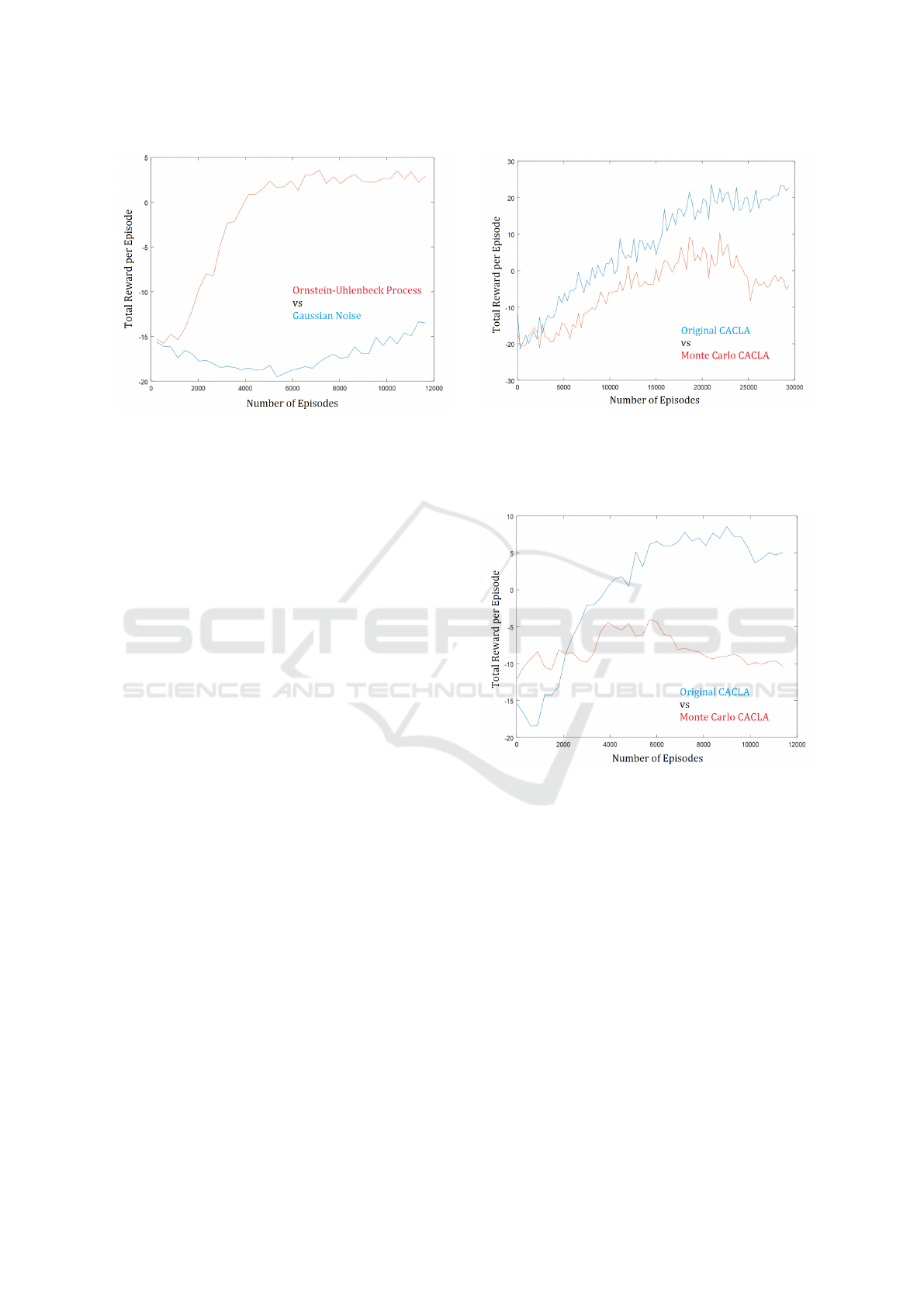
Figure 3: Results of the competition between CACLA with
Gaussian exploration (g
0
t
) and CACLA with OUP-based ex-
ploration (z
t
). The graphs are averaged over ten different
random initializations. The standard deviation of the noise
g
t
was gradually decreased from 0.2 to 0.02.
was used. The signal g
0
t
is scaled such that it has the
same standard deviation as the signal z
t
. An identical
experiment was conducted where the raw g
t
was used
instead of g
0
t
. The result of this experiment is very
similar and thus not reported in this paper.
It can be seen that the total reward of CACLA with
Gaussian exploration decreases initially. This could
be due to more frequent eliminations through the im-
proving marksmanship of CACLA with OUP-based
exploration. By letting experiments run for a longer
time it can be observed that CACLA with Gaussian
exploration is able to converge to a similar final per-
formance as CACLA with OUP-based exploration.
However, CACLA with Gaussian exploration would
take an order of magnitude more time to do so.
Due to the strong result, all of the algorithms in
the following sections were designed with the OUP-
based exploration.
4.2 Monte Carlo CACLA
In Figure 4 and Figure 5, it can be seen that the
original CACLA strongly outperforms MC-CACLA
with the exception of the first 2000 episodes. Since
the MC-CACLA uses more memory and uses the ac-
curate Return R
t
, one would intuitively expect MC-
CACLA to be superior. One reason of its worse
performance is that Monte Carlo learning techniques
have a larger variance in their updates than TD-
learning algorithms. Another reason could be the
spiking rewards that produce a Return that locally re-
sembles a step-function over time. The Critic, ap-
proximating this stepping Return, might not be suffi-
ciently precise to discriminate between the surround-
Figure 4: Results of the competition between the Monte
Carlo version of CACLA and the original CACLA. The
graphs are averaged over five different random initializa-
tions. The standard deviation of the noise g
t
was gradually
decreased from 0.5 to 0.01.
Figure 5: Results of the competition between the Monte
Carlo version of CACLA and the original CACLA. The
graphs are averaged over ten different random initializa-
tions. The standard deviation of the noise g
t
was gradually
decreased from 0.2 to 0.02.
ing time steps before and after the reward spike. This
would lead to positive or negative differences between
the Value and the Return. This would then disturb
the Actor’s learning rule that relies on the difference
R
t
−V
t
(s
t
). This problem of the algorithm was then
looked for in the original CACLA as well. The prob-
lem was found to be theoretically possible in the orig-
inal CACLA (described in section 2.4), but in a more
benign way, the deviation of the Critic around a spike
would be smaller in the original CACLA. In section
2.4 a possible solution to this problem was described.
The following section presents the results of this so-
lution.
ICAART 2018 - 10th International Conference on Agents and Artificial Intelligence
58
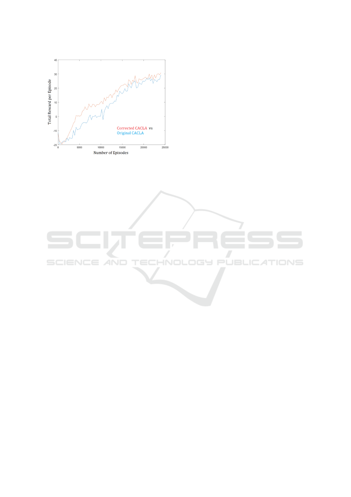
Figure 6: Results of the competition between the Corrected
CACLA and the original CACLA algorithm. The graphs
are averaged over ten different random initializations. The
standard deviation of the noise g
t
was gradually decreased
from 0.5 to 0.01.
4.3 Corrected CACLA
In Figure 6, it can be seen that the Corrected CA-
CLA on average outperforms the original CACLA.
The averages of the total rewards from the first un-
til the last episode were compared. The Corrected
CACLA algorithm performed better for ten out of ten
random initializations which resulted in a p-value of
2
−10
. The strongest difference in performance is be-
tween the 5000th and the 10,000th episode. Towards
the end of the graph the two algorithms converge to-
wards the same strategy and the same performance.
The Corrected CACLA algorithm is constructed such
that it has an advantage when there are negative re-
ward spikes as explained in section 2.4. This advan-
tage is confirmed by these results. Later, once the
agents learned to increase their flight safety such that
there are less negative reward spikes, the Corrected
CACLA loses its advantage. This advantage might
prevail in a different environment where the negative
reward spikes do not disappear over time.
5 CONCLUSIONS
All of the algorithms were tested by competing in our
aerial combat environment. Our results show that sub-
stituting the original Gaussian noise in CACLA with
the OUP leads to a strongly improved exploration of
actions and better performance of the algorithm. This
improvement is to be expected in environments where
the optimal action sequences are temporally corre-
lated, which is typical for continuous environments.
The results also showed that MC-CACLA performs
worse than the original CACLA algorithm. More
work on a Monte Carlo version of CACLA would
need to be done. One possible cause of the poor per-
formance is that the temporal inaccuracy of the Critic
disturbs the learning rule of the Actor. The same prob-
lem was found in the original CACLA but to a much
lesser degree. This problem appears when spiking re-
wards are given. We solved this problem in CACLA
by adding a third MLP that is used to predict the log-
arithm of the absolute error of the Critic. The learn-
ing rule of the Actor was then adapted such that it is
trained only when the TD-error is larger than the es-
timated absolute error of the Critic. This algorithm
was described in detail in section 2.4. The results
show that this approach can indeed improve the per-
formance over the original CACLA algorithm. This
result is remarkable because the Actor in the Cor-
rected CACLA is trained less often than in the original
CACLA. However our Corrected CACLA likely only
has an advantage in environments where negative re-
ward spikes occur.
In future research a similar algorithm could be
developed that also improves CACLA’s performance
when there are mostly positive reward spikes. Fur-
thermore, extending these algorithms by a learnable
model that is used to plan ahead at multiple temporal
resolutions could strongly improve the final perfor-
mance of agents in this aerial combat environment.
This is left as future research.
REFERENCES
Barto, A. (1984). Neuron-like adaptive elements that can
solve difficult learning control-problems. Behavioural
Processes, 9(1).
Bom, L., Henken, R., and Wiering, M. (2013). Rein-
forcement learning to train Ms. Pac-Man using higher-
order action-relative inputs. In Proceedings of IEEE
International Symposium on Adaptive Dynamic Pro-
gramming and Reinforcement Learning : ADPRL.
Ernest, N., Carroll, D., Schumacher, C., Clark, M., Cohen,
K., and Lee, G. (2016). Genetic fuzzy based artificial
intelligence for unmanned combat aerial vehicle con-
trol in simulated air combat missions. J Def Manag,
6(144):2167–0374.
Jensen, J. and Valdemar, L. (1906). Sur les fonctions con-
vexes et les in
´
egalit
´
es entre les valeurs moyennes.
Acta mathematica, 30(1):175–193.
Koutn
´
ık, J., Cuccu, G., Schmidhuber, J., and Gomez, F.
(2013). Evolving large-scale neural networks for
vision-based reinforcement learning. In Proceedings
of the 15th annual conference on Genetic and evolu-
tionary computation, pages 1061–1068. ACM.
Lillicrap, T., Hunt, J., Pritzel, A., Heess, N., Erez, T., Tassa,
Y., Silver, D., and Wierstra, D. (2015). Continu-
Actor-Critic Reinforcement Learning with Neural Networks in Continuous Games
59

ous control with deep reinforcement learning. arXiv
preprint arXiv:1509.02971.
Mnih, V., Kavukcuoglu, K., Silver, D., Graves, A.,
Antonoglou, I., Wierstra, D., and Riedmiller, M.
(2013). Playing atari with deep reinforcement learn-
ing. arXiv preprint arXiv:1312.5602.
Prokhorov, D. and Wunsch, D. (1997). Adaptive critic
designs. IEEE transactions on Neural Networks,
8(5):997–1007.
Rumelhart, D., Hinton, G., and Williams, R. (1988). Learn-
ing representations by back-propagating errors. Cog-
nitive modeling, 5(3):1.
Sutton, R. and Barto, A. (1998). Reinforcement learning:
An introduction, volume 1. MIT press Cambridge.
Tesauro, G. (1995). Temporal difference learning and TD-
gammon. Communications of the ACM, 38(3):58–68.
Uhlenbeck, G. and Ornstein, L. (1930). On the theory of
the brownian motion. Physical review, 36(5):823.
van Hasselt, H. and Wiering, M. (2007). Reinforcement
learning in continuous action spaces. In Approximate
Dynamic Programming and Reinforcement Learning,
2007. ADPRL 2007. IEEE International Symposium
on, pages 272–279.
Watkins, C. and Dayan, P. (1992). Q-learning. Machine
learning, 8(3):279–292.
Wiering, M. and Van Otterlo, M. (2012). Reinforcement
Learning State-of-the-Art, volume 12. Springer.
Zeh, J. and Birkmire, B. (2014). Advanced framework for
simulation, integration and modeling (AFSIM) ver-
sion 1.8 overview. Wright Patterson Air Force Base,
OH: Air Force Research Laboratory, Aerospace Sys-
tems.
ICAART 2018 - 10th International Conference on Agents and Artificial Intelligence
60
