Saliency based Adjective Noun Pair Detection System

Marco Stricker

, Syed Saqib Bukhari

, Damian Borth

and Andreas Dengel

1,2

German Research Center for Artiﬁcial Intelligence (DFKI), Trippstadter Straße 122, 67663 Kaiserslautern, Germany

Technical University of Kaiserslautern, Gottlieb-Daimler-Straße 47, 67663 Kaiserslautern, Germany

Keywords:

Saliency Detection, Human Gaze, Adjective Noun Pairs, Neural Networks.

Abstract:

This paper investigates if it is possible to increase the accuracy of Convolutional Neural Networks trained

on Adjective Noun Concepts with the help of saliency models. Although image classiﬁcation reaches high

accuracy rates, the same level of accuracy is not reached for Adjective Noun Pairs, due to multiple problems.

Several beneﬁts can be gained through understanding Adjective Noun Pairs, like automatically tagging large

image databases and understanding the sentiment of these images. This knowledge can be used for e.g. a

better advertisement system. In order to improve such a sentiment classiﬁcation system a previous work

focused on searching saliency methods that can reproduce the human gaze on Adjective Noun Pairs and found

out that “Graph-Based Visual Saliency” belonged to the best for this problem. Utilizing these results we

used the “Graph-Based Visual Saliency” method on a big dataset of Adjective Noun Pairs and incorporated

these saliency data in the training phase of the Convolutional Neural Network. We tried out three different

approaches to incorporate this information in three different cases of Adjective Noun Pair combinations. These

cases either share a common adjective or a common noun or are completely different. Our results showed only

slight improvements which were not signiﬁcantly better besides for one technique in one case.

1 INTRODUCTION

Image classiﬁcation is an important subject in com-

puter science and can be applied for many different

subjects, e.g. people or object recognition. In to-

day’s time with buzzwords like Big Data where mas-

sive amounts of data is created and saved within a

short period of time a manual description of such im-

ages is not possible. Therefore an automatic way is

needed, so that the images in these databases can be

tagged and searching through them or generally work-

ing with them is possible. Currently methods work re-

ally well on general image classiﬁcation, as it can be

seen in the ImageNet challenge (Russakovsky et al.,

2015), but they don’t achieve the same level of per-

formance on specifying these images with adjectives,

such as “cute dog” for example, as it can be seen

in (Chen et al., 2014b) or (Chen et al., 2014a), who

tried to build a classiﬁer for this problem. (Jou et al.,

2015) also tried to solve this by using a multilingual

approach and achieved better results, which are still

not on the same level as the general image classiﬁca-

tion. Thus the classiﬁcation of such Adjective Noun

Pairs a.k.a ANPs still needs to be improved. One of

the difﬁculties such methods need to face are objec-

tivity vs. subjectivity, e.g. a “damaged building” is

objectively damaged by a hole in a wall while decid-

ing if a baby is cute is a subjective opinion depen-

dent on the user. The other difﬁculty are localizable

vs. holistic features. The feature hole in a damaged

building is localized in a ﬁxed sub-part of the image.

On the other hand to estimate if a landscape is stormy

the whole image needs to be taken into account. Sam-

ple images of this conﬂict can be found in Figure 1.

Another problem in ANP classiﬁcation is the tagging

of images. First, there may be multiple ANPs in one

image, e.g. an ANP of “stormy landscape” probably

also includes the ANP “dark clouds”, which makes it

more difﬁcult to create a ground truth dataset. This is

furthermore increased by the second problem of syn-

onyms, e.g. the ANP image of a “cute dog” can also

be used for “adorable dog”. Nevertheless (Borth et al.,

2013) created an ANP dataset which we will be using

in this paper. A short description of this ANP dataset

can be found in section 2.

In a previous work (Al-Naser et al., 2015) the authors

investigated these problems with an Eye-Tracking

experiment. In detail they asked if the participant

agreed with a certain ANP e.g. “beautiful landscape”

and recorded their eye-gaze data. An example of

how such eye gaze data look like can be seen in

Figure 1. Under the sample images the heat maps are

Stricker, M., Bukhari, S., Borth, D. and Dengel, A.

Saliency based Adjective Noun Pair Detection System.

DOI: 10.5220/0006578303870394

In Proceedings of the 10th International Conference on Agents and Artiﬁcial Intelligence (ICAART 2018) - Volume 2, pages 387-394

ISBN: 978-989-758-275-2

387

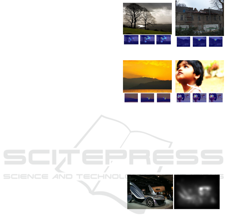
visualizing the most focused regions for the cases of

agreement between user and ANP, disagreement and a

combination of both. Each ground truth is the combi-

nation of all participants who were of the same opin-

ion regarding this ANP. But only 8 out of 3000 ANPs

(Borth et al., 2013) were used with just 11 human

participants. A manual creation of such a database

with all ANPs is not feasible. Following this problem

(Stricker et al., 2017) investigated if there are saliency

models capable of recreating the human gaze. They

found out, that there are models which are better than

other in handling this task. Figure 2 shows an image

with its corresponding saliency map to visualize how

such a saliency map may look like.

There are also similar works which are trying differ-

ent approaches to detect the sentiment of an image or

text. Some examples include (Cao et al., 2016), (You

et al., 2016) or (Vadicamo et al., 2017)

This paper focuses on utilizing these results by us-

ing the saliency methods on the aforementioned larger

dataset of ANPs (without eye-gaze data), which is de-

scribed in section 2, as a preprocessing step. The im-

ages are then ﬁltered and unsalient regions are dis-

carded under the assumption that these new images

will improve the accuracy of our saliency based ANP

detection system. We trained a deep learning CNN

with these data, which is described in section 3 while

the explanation on how we incorporated the saliency

data is done in section 4. Following this the results

are presented and discussed in section 5. Lastly this

paper ends with a conclusion on our ﬁndings in sec-

tion 6.

2 THE ANP DATASET

In this paper a subset of the Visual Sentiment Ontol-

ogy (Borth et al., 2013) was used. We are now brieﬂy

describing the creation of this dataset.

First of all Plutchnik’s Wheel of Emotions (Plutchik,

1980) was used as an emotional model. It consists

of eight basic emotions and each of them is further

separated into three more. This leads to a total of

24 emotions which are named in table 1. These 24

emotions were used to look for images on Flickr in-

cluding their tags. With this procedure 310k images

and 3M tags were retrieved. The tags were analyzed

by removing stop-words and performing stemming.

Furthermore a ranking of the top 100 tags was cre-

ated by using tag frequency analysis. This resulted

in 1146 distinct tags. As a last preprocessing step

a sentiment value is calculated for each tag so that

all tags have a value from -1 to +1 where negative

numbers represent a negative association and positive

(a) Stormy Landscape

(Holistic, Objective)

(b) Damaged Building (Lo-

calized, Objective)

(Holistic, Subjective)

(d) Cute Baby (Localized,

Subjective)

Figure 1: This ﬁgure shows the four ANP samples: “stormy

landscape”, “damaged building”, “beautiful landscape” and

“cute baby”. Below these images are the three forms of

ground truth. The order is from left to right: disagreement,

agreement and combination. Not all ground truth images

are showing eye gaze data. This is because for that image no

participant disagreed or agreed with the ANP and therefore

no gaze data was recorded in combination with this answer.

Furthermore these four images are showing the problems of

objective vs. subjective ANPs and holistic vs. localizable

ANPs.

Figure 2: An image of an “amazing car” with its corre-

sponding saliency map calculated by “Graph-Based Visual

Saliency”.

numbers represent a positive association. After this

preprocessing the ANPs can be constructed by com-

bining adjectives with nouns, in order to give neutral

nouns a sentiment value. The resulting ANPs are now

analyzed to ﬁnd ANPs which are an already existing

concept, like “hot” + “dog”. These images were re-

moved. Furthermore if the values of the noun and the

adjective contradict each other the noun will get the

value of the adjective. This was done in order to solve

cases like “abused” + “child”. Otherwise the senti-

ment value of the ANP is just the sum of both. Lastly

rare constructs are removed.

Two problems the dataset is facing are false pos-

itive and false negative. False positive means that

an image is labeled with an ANP but doesn’t show.

ICAART 2018 - 10th International Conference on Agents and Artiﬁcial Intelligence

388

Table 1: The 24 emotions divided into eight basic emotions

as described by Plutchnik’s Wheel of Emotions.

Ecstasy Joy Serenity

Admiration Trust Acceptance

Terror Fear Apprehension

Amazement Surprise Distraction

Grief Sadness Pensiveness

Loathing Disgust Boredom

Rage Anger Annoyance

Vigilance Anticipation Interest

it, e.g. an image which clearly shows a ﬂower, but

is labeled as “abandoned area”. This problem was

analyzed with the Amazon Mechanical Turk which

showed that 97% of the labels are correct. False nega-

tive represents the problem that an image is not tagged

with a label although it clearly shows it. Unfortu-

nately this problem is still an open issue and could

only be minimized.

As earlier stated we used a subset of the aforemen-

tioned Visual Sentiment Ontology. To show if our ap-

proach can really improve the performance for ANP

speciﬁc tasks we created three subsets as shown in ta-

ble 2. The ﬁrst one “Normal” consists of ten classes

where no adjective or noun appears more than once.

“Same Adjective” consists of ten classes with the

same adjective, namely “amazing”. Similarly “Same

Noun” consists of ten classes sharing the same noun

“car”. The goal of these three test cases is to show if

our modiﬁed network will perform better at learning

certain adjectives or different kinds of nouns.

3 DEEP LEARNING CLASSIFIER

FOR ANPS

To train the deep learning classiﬁer on the dataset we

used Tensorﬂow as a framework. Within it we trained

a simple convolutional neural network. Since the goal

of this paper is not to develop a state of the art clas-

siﬁer for ANPs but to investigate the effects of in-

cluding saliency data, a simple network sufﬁces for

this proof of concept. We want to check if saliency

data is capable of increasing the accuracy. Therefore

we have taken a simple convolutional neural network

as described by Tensorﬂow’s introduction to convolu-

tional neural networks (Tensorﬂow, 2017).

We are now going to brieﬂy describe the architecture.

The proposed network was made in order to solve

the CIFAR-10 classiﬁcation problem (Krizhevsky and

Hinton, 2009). This means that the network is capable

of classifying 32x32 pixels into ten categories. These

categories are: airplane, automobile, bird, cat, deer,

dog, frog, horse, ship and truck. Furthermore the ac-

curacy of this network is about 86%.

This is also our reason for choosing this network. It

achieves a good performance on a similar problem,

which is categorizing images into ten classes. Nev-

ertheless our classes are more complex because now

the network doesn’t need to learn ten simple concepts

(nouns) which are clearly different from each other

but also needs to learn an adjective description. Fur-

thermore our classes with which we test the network

are not always distinct from each other. This can

be best seen in our test case for similar nouns where

the network needs to learn to distinguish between an

“amazing car” and an “awesome car”. Even humans

would not be able to reliably perform this task due

to many difﬁcult problems. These problems are, that

such adjective are sometimes subjective, e.g. what

person A thinks might be beautiful might be ugly for

person B. Furthermore many ANPs are similar to each

other like the earlier example of “amazing” and “awe-

some” where both can be used to describe the same

object. Unfortunately this dataset doesn’t support that

a single image is described by multiple ANPs. This

also includes the problem that an image shows a ﬁt-

ting ANP but we don’t have it included in our list of

ANPs. This leads to the conclusion that our accuracy

will be far worse than the accuracy on the CIFAR-10

dataset.

The proposed network as it can be seen in ﬁgure 3 (a),

consists of three major steps, which will be described

in detail later. First the input images are read and pre-

processed. Secondly a classiﬁcation will be done on

the images. Lastly the training is done to compute all

variables.

3.1 Training Preparation

The images are simply read from a binary ﬁle. After

that the proposed network crops the images to 24x24

pixels. But we skip this step, because our testset per-

formed better with images size being 32x32 pixels.

All other steps were not modiﬁed. Therefore our sec-

ond step was to whiten the images so that the model

is insensitive to dynamic range.

3.2 Classiﬁcation

The layers of the CNN for classiﬁcation are build as

shown by ﬁgure 3 (a).

The layers take over different tasks. ConvX rep-

resents a convolution layer which uses a rectiﬁed lin-

ear activation function. PoolX takes over the pooling

task by using maximum values. NormX performs a

normalization. LocalX are fully connected layers. Fi-

Saliency based Adjective Noun Pair Detection System

389

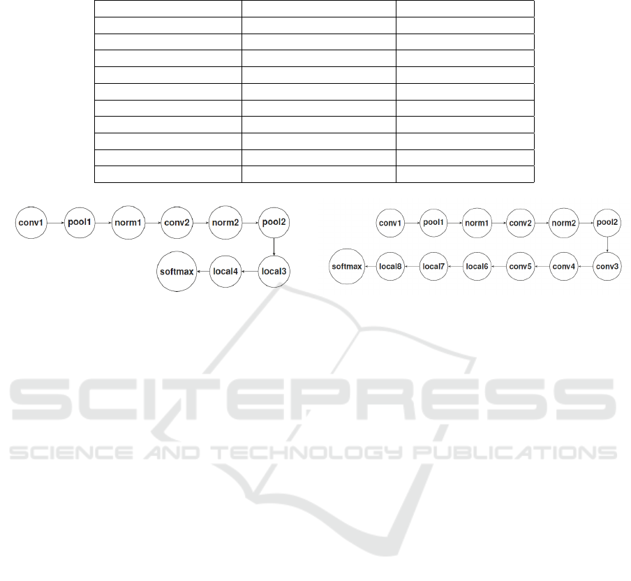
Table 2: A list of all ten classes for each subset. The number after the class marks how many images belong to each of the

classes.

Normal Same Adjective Same Noun

Abandoned Area (799) Amazing Baby (644) Abandoned Car (844)

Active Child (958) Amazing Cars (959) Amazing Car (959)

Adorable Cat (741) Amazing Dog (787) Antique Car (985)

Aerial View (955) Amazing Flowers (840) Awesome Car (876)

Amateur Sport (603) Amazing Food (918) Beautiful Car (825)

Amazing Cars (959) Amazing Girls (834) Big Car (967)

Ancient Building (822) Amazing Nature (835) Classic Car (963)

Antique Airplane (738) Amazing People (923) Cool Car (989)

Arctic Ice (842) Amazing Sky (899) Exotic Car (935)

Artiﬁcial Leg (454) Amazing Wedding (882) Large Car (961)

(a) The ﬁrst CNN

(b) The second CNN

Figure 3: The two CNN architectures we have used. The second one has more convolutional layers.

nally softmax is a linear transformation.

We also trained a second network, as shown in ﬁgure

3 (b) which has three more convolutional layers and a

third fully connected layer.

3.3 Training

The model was trained using gradient descent. We

trained this model on the different datasets as de-

scribed in section 2. We used 80% of the images

for training and 20% for testing. During training we

reached 350 Epochs and stopped after running 5000

batches with a size of 128. Furthermore our training

set contained the three different approaches of incor-

porating saliency data and one set without saliency

data in order to get accuracy values against which we

can compare later.

4 INCORPORATING SALIENCY

DATA

The CNN from section 3 is for the most cases the

same and we tried different approaches how to incor-

porate the saliency data. All the different approaches

share the same preprocessing which will be now de-

scribed.

First of all we used all the images and applied the

saliency method “Graph-Based Visual Saliency” a.k.a

GBVS (Harel et al., 2006) on them. We decided to use

GBVS as a saliency method because it performed as

one of the best saliency methods overall for detect-

ing important regions on ANPs according to (Stricker

et al., 2017).

The approach of GBVS is inspired by biology. It

forms activation maps on certain feature channels and

normalizes them to highlight conspicuity. Further-

more all images were resized to 32x32 pixels. This

leads to two sets of images. The ﬁrst one contains all

original images at size 32x32 pixels while the second

one contains all saliency maps at size of 32x32 pixels.

We have in total investigated three ways of incorporat-

ing these saliency maps into the image in order to help

the network to concentrate on the important regions.

The ﬁrst method is a simple masking method and the

second one is exploiting tensorﬂows option to train

on four dimensional images with an alpha value addi-

tionally to the standard RGB channel. This approach

does have two possibilities of incorporating saliency

data. Lastly we also used a way of cutting out the im-

portant parts of the image to train on a smaller image

which only contains the relevant data.

4.1 Simple Salient Masking Filtering

The simple masking method compares the original

image with the saliency map pixel per pixel. It creates

the new image with the condition, that if the value of

the saliency map is greater than 127, which is half of

ICAART 2018 - 10th International Conference on Agents and Artiﬁcial Intelligence

390

the maximum of 255, the corresponding pixel’s RGB

data in the original image will be taken to the new im-

age without modiﬁcation. Otherwise the RGB value

in the new image will be (0, 0, 0). This means that

if the saliency map’s value on position x1, y1 is e.g.

223, then the RGB value of the original image at po-

sition x1, y1 will be written at the new image’s posi-

tion x1, y1. But if the value at position x2, y2 in the

saliency map is 100, then the value of new image at

position x2, y2 will be zero on all three colour chan-

nels. We didn’t experiment with values different from

127, because another approach showed better results

and was therefore more interesting to investigate.

4.2 Exploiting the Salient Alpha

Channel Filters

Tensorﬂow offers the option to deﬁne how many di-

mensions each image has on which the network will

train. Currently it only supports the dimensions one

to four. One means a simple image where each pixel

has the value of zero to 255 e.g. something like a

greyscale map, like our saliency map. Two would be

the same including the alpha channel. Three is the

standard way of RGB and four is RGB with an alpha

channel.

We create the image on which the network will train

by taking the original image and copying all RGB val-

ues one to one. Setting the alpha value is done in two

different ways, where both are using the saliency map

to calculate the alpha value:

• The ﬁrst possibility is to simply take the saliency

map. Each value in the saliency map is a single

number ranging from zero to 255. This ﬁts the

value range of the alpha channel. Therefore we

simply copy the value from the saliency map and

set it as the alpha value.

• For the second possibility we utilize the ﬁndings

from (Stricker et al., 2017). One of the impor-

tant contributions was observing that the perfor-

mance of saliency methods like GBVS signiﬁ-

cantly increased after binarizing the saliency map

with a threshold determined by Otsu’s method

(Otsu, 1975). Thus we binarized the saliency map

and set the alpha value to 255 if the correspond-

ing saliency map pixel had the value one. If the

saliency map pixel value is zero we also set the

corresponding pixel’s alpha value to zero.

4.3 Salient Region Patch Extraction

Lastly we investigated the effects of cutting out the

important regions of an image and patching them to-

gether to create a new smaller image on which the

network learns.

In detail we searched for the n most important regions

of the image. In our case we set n to four. In a naive

approach those n regions can be found easily. We

have our saliency map from which we can derive the

salient regions. Therefore in a simple way we could

have just taken the pixels where we found the n high-

est values. But this does have one major problem.

How can we assure that we have taken points that

actually represent different regions of the image and

not just the pixels on position (x,y), (x+1,y), (x,y+1)

and (x+1,y+1). It is highly probable that if pixel (x,y)

has the highest value, then the surrounding pixels will

have a very high value themselves. We need to avoid

the case where we choose pixels right beside each

other to achieve our goal of covering a big part of

the image. Therefore we cannot take the ﬁrst n pixels

with the highest value or choose them randomly. Fig-

ure 4 illustrates this problem.

This problem can be solved by the following proce-

dure. We deﬁne a set A which contains all pixels

where each pixel has maximum value. We will ex-

plain later how we build the set in detail. After that

we take a look at all possible subsets of A with length

n. This means that each subset is a possible solution to

our problem. For all subsets we calculate the distance

between all points. As a distance measure we used the

euclidean distance. Then we sum up the length of all

distances. The solution to our problem is the subset

where this sum is maximal, because this will give us

the points whose distance is maximal to each other. In

a more formal way we choose the subset which max-

imizes the following sum:

∑

i=0

∑

j=i+1

distance(p

, p

) (1)

Figure 4 also showcases this solution.

Another problem is how to calculate the set A. The

problem lies in how to deﬁne a maximal value, which

is the condition for the points inside set A. If we take

a look at ﬁgure 5 we can see again the same image as

before, where there are again three red circles which

illustrate the three salient regions. This time they are

ﬁlled with three colours. Red, orange and yellow. If

the circle is ﬁlled with red, this means that all pix-

els inside it have the value of 253 to 255 according

to the saliency map. An orange ﬁlling represents the

values 250 to 252. Lastly the yellow points represent

a value between 247 and 249. It is obvious that set

A needs to include pixels from all three circles. The

value range is close enough (247 to 253 are only 6

points difference) to be considered maximal. Nev-

ertheless such a case is possible were such a salient

region may have an upper bound which is lower than

Saliency based Adjective Noun Pair Detection System

391

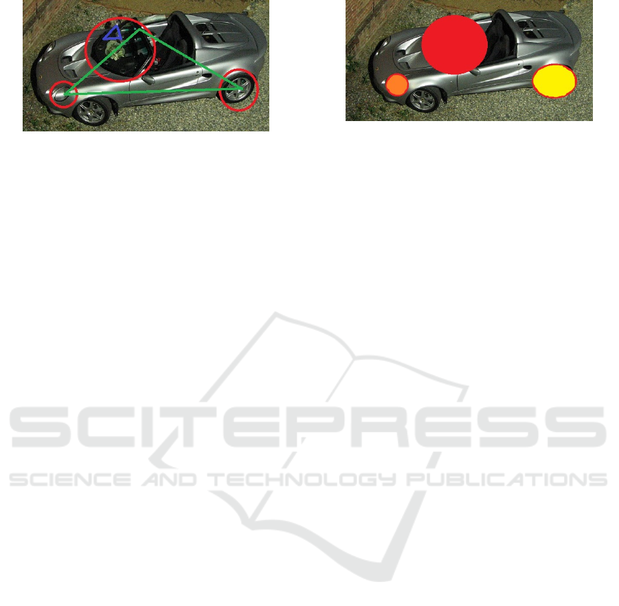
Figure 4: This image shows a car where multiple areas have

been marked as salient (marked by the red circle). To cover

the whole image we want to choose a part of the image from

the three shown salient regions, meaning we want to include

the tire, lights and window, instead of choosing to cut out

the tire multiple times. This image also illustrates the solu-

tion to this problem . We take a look at all subsets and con-

nect all points inside a subset with each other. This results

in multiple triangles, e.g. the green and the blue one. All

points of the blue triangle are inside the same salient region

and therefore the sum of the lines is rather small. Instead

the green triangle who has points in all salient regions has

a higher sum of the lines. Thus deciding to take the points

deﬁned by the green triangle is the better choice.

the maximum value in the whole image. Therefore we

cannot take the absolute best value in the whole image

and look only for pixels with the same one. Then we

would only take the red pixels and couldn’t achieve

the big coverage of the image.

Our solution to this problem was to take a sorted list

of all the saliency values with descending order. Then

we took the nth element and looked at its value v.

Now we need to deﬁne a lower bound depending of

v where all pixels with a higher value than v are con-

sidered to be a maximal for set A. We chose the lower

bound to be 10% smaller than v. Therefore our set A

is deﬁned by:

A = {p|p ≥ (t ∗ 0.9)∀p ∈ P} (2)

With t being the nth highest value over all pixels and

P containing all pixels.

It is not advised to choose a high percentage for

this, because we are looking at all possible subsets

of length n of A the number of subsets we need to

check drastically increases which results in a signiﬁ-

cant longer computation time.

After this preprocessing we have a set of n pixels.

We set the pixel to be the center of a 8x8 pixels big

sub-part of the image. Because we are doing this for

four pixels we will get four 8x8 pixels sub-parts of the

image. These four sub-parts are cut out and then com-

bined to create the new image on which the network

will train.

Figure 5: This image showcases the problem of how to de-

ﬁne the set A. Red pixels inside the red circle have a value

of 253 to 255. Orange pixels inside the red circle have a

value of 250 to 252. Yellow pixels inside the red circle have

a value of 247 to 240. It is obvious that the set A needs to

consider all red, orange and yellow pixels as a pixel with

maximal value and not only the red ones.

5 DISCUSSION

We are now going to present the results we have gath-

ered with our methods. Table 3 shows all values for

the ﬁrst network. The columns represent the differ-

ent datasets which were used. These are “Normal”,

“Same Adjective” and “Same Noun”. “Normal” con-

sists of ten classes where each classes adjective and

noun is different from each other. Contrary to this

“Same Adjective” consists of ten classes all contain-

ing the same adjective but different nouns. Similar to

this “Same Noun” consists of ten classes all contain-

ing the same noun but different adjectives.

The rows are showing which technique was used to

train the CNN. “Standard” means using the CNN as

described in section 3 on unﬁltered images, while the

other rows represent the methods used for ﬁltering the

images, as described in section 4.

Following these results, we again tried this

method with using the deeper network as shown in

section 3. The results can be seen in table 4.

Taking the not enhanced images, as seen in the re-

sults table of the standard row, as a baseline, we can

see that the techniques of simple masking and patches

have failed to increase the accuracy and performed

worse in both CNNs.

The patches method probably failed due to the rea-

son that the saliency map did not create multiple dis-

connected areas on the images, as it can be seen in

ﬁgure 4 but instead created a connected area, where

high salient regions are close to each other. Further-

more those high salient regions mostly lie close to

each other, therefore the method to patch the image

often took similar parts of the image and threw away

important information. An example of how such a

saliency map looks like can be seen in ﬁgure 2. Fur-

thermore ﬁgure 6 shows some example images and

their corresponding images as created by the patches

ICAART 2018 - 10th International Conference on Agents and Artiﬁcial Intelligence

392

Table 3: Accuracy’s on the different datasets “Normal”, “Same Adjective” and “Same Noun” using the standard CNN and the

different methods of incorporating the saliency datas.

Saliency Data Incorporation Normal Same Adjective Same Noun

Standard 0.404 0.241 0.173

Simple Masking 0.239 0.220 0.137

Alpha Value (Binarized) 0.132 0.343 0.181

Alpha Value (Not Binarized) 0.333 0.32 0.163

Patches 0.226 0.197 0.109

Table 4: Accuracy’s on the different datasets “Normal”, “Same Adjective” and “Same Noun” using a CNN with more layers

and the different methods of incorporating the saliency datas.

Saliency Data Incorporation Normal Same Adjective Same Noun

Standard 0.411 0.327 0.171

Simple Masking 0.255 0.208 0.140

Alpha Value (Binarized) 0.413 0.338 0.21

Alpha Value (Not Binarized) 0.421 0.338 0.178

Patches 0.252 0.196 0.13

method. These images are highlighting this problem.

The simple masking method may have failed due

to the same reason. Because pixels are either taken or

completely disregarded some important information

has been lost.

On the other hand the methods exploiting the alpha

value have shown some improvements for the stan-

dard CNN, with the exception of the “Normal” case.

There we can see a big drop in accuracy of 30%. For

the case of “Same Noun” we can see a tiny improve-

ments in the binarized alpha method while the results

for the not binarized method showed slightly wors-

ened. On the other hand both methods increased the

accuracy in the “Same Adjective” case by 8% - 10%.

Therefore for this network, the use of saliency

guided data, incorporated by the binarized alpha value

method has shown success in the case of using it for

data where the ANPs are not distinct from each other,

e.g. they share either adjectives or nouns. If they

don’t share adjectives or nouns, the approach doesn’t

improve the accuracy.

In the case of the deeper CNN, we can see some dif-

ferences compared to the standard one. First of all

the big accuracy loss in the “Normal” case does not

happen and it even slightly increased, for both alpha

value methods, compared to the not saliency guided

method. Nevertheless the deeper architecture of the

network has also improved the accuracy of the not

saliency guided method in the “Same Adjective” case.

While both alpha value methods are still better, the

improvements are now only small by 1%. Contrary

to this, the new architecture did not increase the accu-

racy for the not saliency guided method in the “Same

Noun” case but it did improve the accuracy’s for the

saliency guided methods. Therefore now both alpha

value methods are better by a small value. The not bi-

narized one is better by only 0.7% while the binarized

one showed improvements of 3.9%.

Therefore in the deeper CNN, both alpha value meth-

ods showed slight improvements in all cases. The bi-

narized one was better in the “Same Noun” case com-

pared to the not binarized one while the not binarized

one was better in the “Normal” case.

We think that the alpha value methods are better than

the other saliency guided methods, because the other

methods strictly remove information, while the alpha

methods only guide the CNN as to where important

regions may be but does not remove the information

of the other regions and instead only reduces their im-

pact.

Lastly we also performed a signiﬁcance test on the

accuracy’s of the deeper network, to check if the ac-

curacy’s are also signiﬁcantly better. We compared

the results in each of the cases “Normal”, “Same Ad-

jective” and “Same Noun”. In each of the cases we

checked if the accuracy of “Alpha Value (Binarized)”

and “Alpha Value (Not Binarized)” are signiﬁcantly

better than the accuracy of the “Standard” way.

We conducted a t-test with our ﬁndings. Our results

show that only the accuracy’s of “Alpha Value (Bi-

narized)” in the case of “Same Noun” is signiﬁcantly

better than the standard model. The two-tailed P value

equals 0.0024 in this case.

6 CONCLUSION

In this paper we investigated the impact of saliency

data on CNNs trained to recognize a small set of

ANPs. This set of ANPs was divided into three

Saliency based Adjective Noun Pair Detection System

393

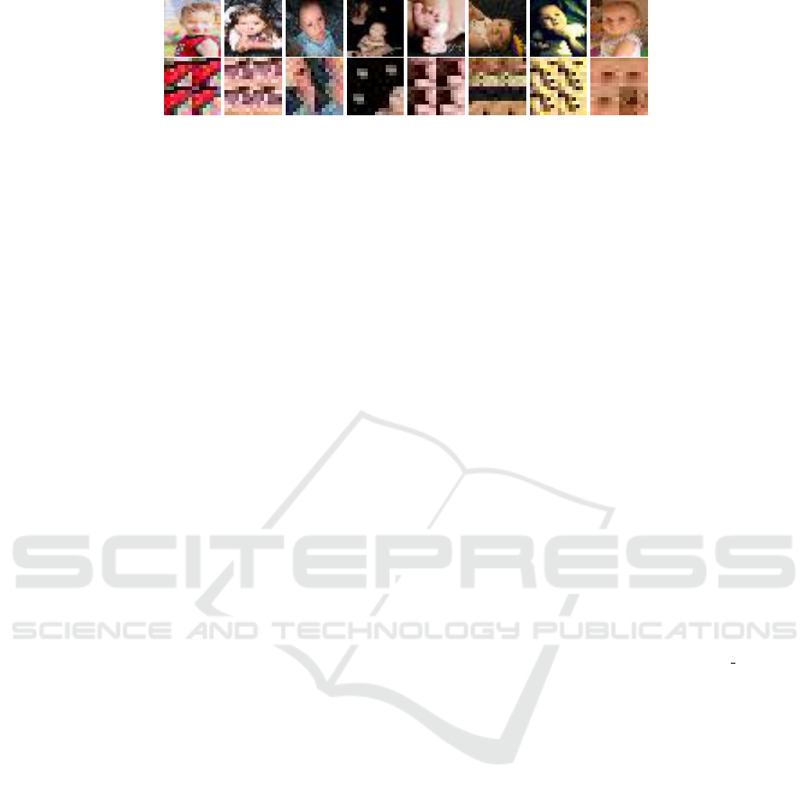
Figure 6: This ﬁgure shows eight example images from the ANP “amazing baby” in the upper row. The lower row shows

their corresponding images as they are created by the patches method. (The patched image belongs to the image above it).

This highlights the problem of the method to create those patched images. Namely that it is not capable of selecting distinct

areas but instead very similar ones are used.

categories, “Normal”, “Same Adjective” and “Same

Noun”. We found out that our deeper network showed

some slight improvements by incorporating saliency

data using the alpha value in all three categories.

But these improvements were not statistically signif-

icant besides for the case of “Same Noun” with the

technique of “Alpha Value (Binarized)”. But we ex-

pect better improvements with a bigger dataset, where

each class contains more images. A huge dataset

which satisﬁes all the needs, e.g. the support of mul-

tiple ANPs and synonyms, for this problem. Creating

such a dataset is a difﬁcult and interesting problem

for future work. Furthermore our results are showing

big differences between the different the two CNNs,

which we used. Therefore the impact of different net-

work architectures can also be investigated in future

work to maximize the precision of the approach.

REFERENCES

Al-Naser, M., Chanijani, S. S. M., Bukhari, S. S., Borth,

D., and Dengel, A. (2015). What makes a beautiful

landscape beautiful: Adjective noun pairs attention by

eye-tracking and gaze analysis. In Proceedings of the

1st International Workshop on Affect & Sentiment in

Multimedia, pages 51–56. ACM.

Borth, D., Ji, R., Chen, T., Breuel, T., and Chang, S.-F.

(2013). Large-scale visual sentiment ontology and de-

tectors using adjective noun pairs. In Proceedings of

the 21st ACM international conference on Multime-

dia, pages 223–232. ACM.

Cao, D., Ji, R., Lin, D., and Li, S. (2016). A cross-media

public sentiment analysis system for microblog. Mul-

timedia Systems, 22(4):479–486.

Chen, T., Borth, D., Darrell, T., and Chang, S.-F. (2014a).

Deepsentibank: Visual sentiment concept classiﬁca-

tion with deep convolutional neural networks. arXiv

preprint arXiv:1410.8586.

Chen, T., Yu, F. X., Chen, J., Cui, Y., Chen, Y.-Y., and

Chang, S.-F. (2014b). Object-based visual sentiment

concept analysis and application. In Proceedings of

the 22nd ACM international conference on Multime-

dia, pages 367–376. ACM.

Harel, J., Koch, C., and Perona, P. (2006). Graph-based vi-

sual saliency. In Advances in neural information pro-

cessing systems, pages 545–552.

Jou, B., Chen, T., Pappas, N., Redi, M., Topkara, M., and

Chang, S.-F. (2015). Visual affect around the world:

A large-scale multilingual visual sentiment ontology.

In Proceedings of the 23rd ACM international confer-

ence on Multimedia, pages 159–168. ACM.

Krizhevsky, A. and Hinton, G. (2009). Learning multiple

layers of features from tiny images.

Otsu, N. (1975). A threshold selection method from gray-

level histograms. Automatica, 11(285-296):23–27.

Plutchik, R. (1980). Emotion: A psychoevolutionary syn-

thesis. Harpercollins College Division.

Russakovsky, O., Deng, J., Su, H., Krause, J., Satheesh,

S., Ma, S., Huang, Z., Karpathy, A., Khosla, A.,

Bernstein, M., Berg, A. C., and Fei-Fei, L. (2015).

ImageNet Large Scale Visual Recognition Challenge.

International Journal of Computer Vision (IJCV),

115(3):211–252.

Stricker, M., Bukhari, S. S., Al-Naser, M., Mozafari, S.,

Borth, D., and Dengel, A. (2017). Which saliency

detection method is the best to estimate the human at-

tention for adjective noun concepts?. In ICAART (2),

pages 185–195.

Tensorﬂow (2017). Neural network proposed by tensorﬂow.

https://www.tensorﬂow.org/tutorials/deep cnn.

Vadicamo, L., Carrara, F., Cimino, A., Cresci, S., DellOr-

letta, F., Falchi, F., and Tesconi, M. (2017). Cross-

media learning for image sentiment analysis in the

wild. In Proceedings of the IEEE Conference on Com-

puter Vision and Pattern Recognition, pages 308–317.

You, Q., Luo, J., Jin, H., and Yang, J. (2016). Cross-

modality consistent regression for joint visual-textual

sentiment analysis of social multimedia. In Proceed-

ings of the Ninth ACM International Conference on

Web Search and Data Mining, pages 13–22. ACM.

ICAART 2018 - 10th International Conference on Agents and Artiﬁcial Intelligence

394