Graph-Cut Segmentation of Retinal Layers from OCT Images

Bashir Isa Dodo, Yongmin Li, Khalid Eltayef and Xiaohui Liu

Department of Computer Science, Brunel University, U.K.

Keywords:

Retinal Layer Segmentation, Optical Coherence Tomography, Graph-Cut.

Abstract:

The segmentation of various retinal layers is vital for diagnosing and tracking progress of medication of var-

ious ocular diseases. Due to the complexity of retinal structures, the tediousness of manual segmentation and

variation from different specialists, many methods have been proposed to aid with this analysis. However

image artifacts, in addition to inhomogeneity in pathological structures, remain a challenge, with negative in-

ﬂuence on the performance of segmentation algorithms. Previous attempts normally pre-process the images or

model the segmentation to handle the obstruction but it still remains an area of active research, especially in re-

lation to the graph based algorithms. In this paper we present an automatic retinal layer segmentation method,

which is comprised of fuzzy histogram hyperbolization and graph cut methods to segment 8 boundaries and

7 layers of the retina on 150 OCT B-Sans images, 50 each from the temporal, nasal and centre of foveal re-

gion. Our method shows positive results, with additional tolerance and adaptability to contour variance and

pathological inconsistency of the retinal structures in all regions.

1 INTRODUCTION

Segmentation is the separation of images into more

meaningful information based on similarity or differ-

ence, continuity or discontinuity. Segmentation using

graph cut methods, depends on assignment of appro-

priate weight. The paths obtained by the default short-

est path algorithms, have no optimal way of handling

inconsistencies (such as the irregularity in OCT im-

ages), as thus it sometimes obtains the wrong paths,

which we call the ”wrong short-cuts”. To avoid the

wrong short-cuts, we reassign the weights to promote

the homogeneity between adjacent edges using fuzzy

histogram hyperbolization. In other words, the edges

with high value get higher weights, while those with

low values become lower. The idea behind this is that,

the transition between layers of OCT images which

are from dark to light or vice versa are improved. This

means we can better identify the layers by searching

for the changes or transitions between layer bound-

aries. Additionally, we take into account the transition

between the layers is in most cases very smooth, mak-

ing it quite difﬁcult to segment the layers. Now if we

re-emphasize on this changes, such that they become

clearer, this aids the algorithm in successful segmen-

tation and avoiding wrong short-cuts.

In this paper we take into account the effect of pro-

moting continuity and discontinuity, in addition to

adding hard constraints based on the structure of

retina to segment 7 retinal layers including the Nerve

Fibre Layer (NFL), the Ganglion Cell to Layer-Inner

Plexiform Layer(GCL+IPL), the Inner Nuclear Layer

(INL), the Outer Plexiform Layer (OPL), the Outer

Nuclear Layer to Inner Segment (ONL+IS), the Outer

Segment (OS) and the Retinal Pigment Epithelium

(RPE) by detecting eight (8) layer boundaries. The

locations of these layers and boundaries in an OCT

image are illustrated in Fig.1.

This paper is organized as follows. In Section 2,

we review background information on the Graph-Cut

segmentation method and the previous work in retinal

layer segmentation. Section 3 describes the proposed

segmentation method. Section 4 presents experimen-

tal results on 150 OCT images. Finally conclusions

are drawn in Section 5.

2 BACKGROUND

2.1 The Graph-Cut Method

Graph-Cut is an optimization method used in solving

many image processing and computer vision prob-

lems, as ﬁrst reported by (Seheult et al., 1989), where

the problem is represented as a graph. A graph G is

a pair (ν, ε) consisting of a vertex set ν (referred to

as nodes in 2D or Vertex 3D nested grid) and an edge

Dodo, B., Li, Y., Eltayef, K. and Liu, X.

Graph-Cut Segmentation of Retinal Layers from OCT Images.

DOI: 10.5220/0006580600350042

In Proceedings of the 11th International Joint Conference on Biomedical Engineering Systems and Technologies (BIOSTEC 2018) - Volume 2: BIOIMAGING, pages 35-42

ISBN: 978-989-758-278-3

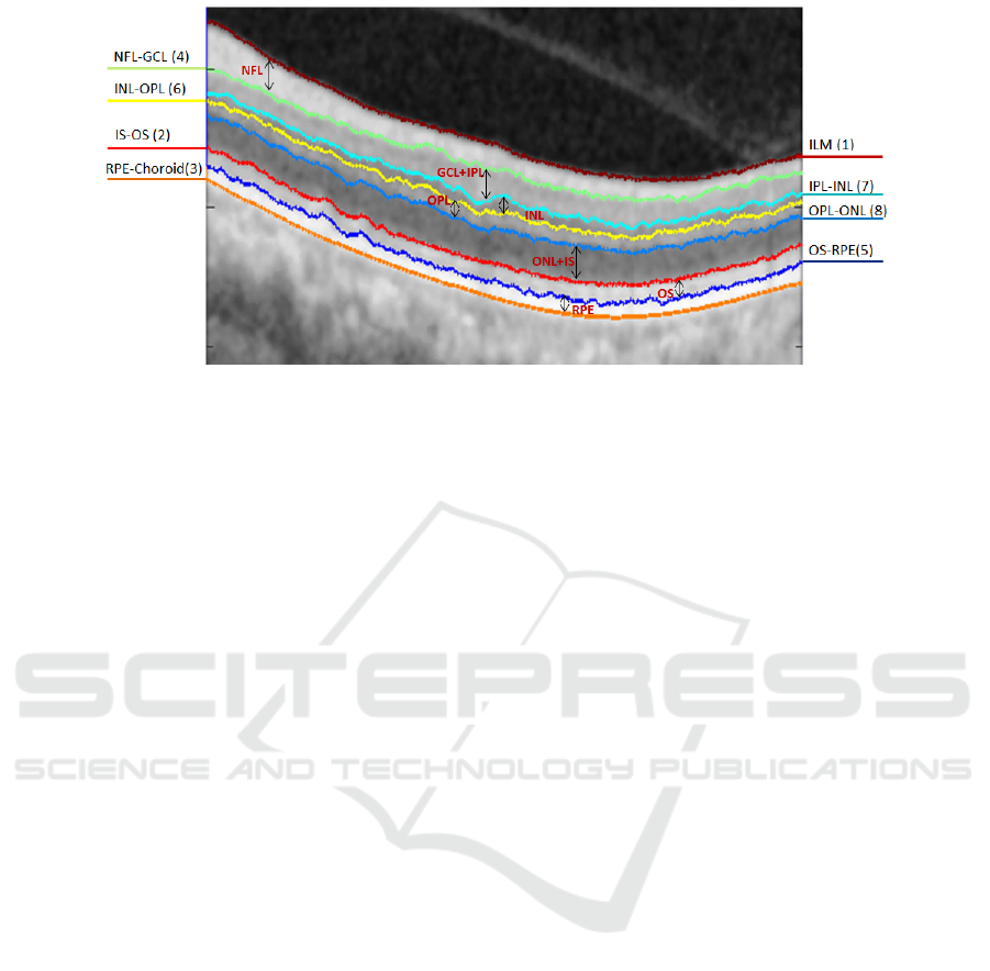
Figure 1: Illustration of the 8 boundaries and 7 retinal layers segmented in the study. The numbers in brackets are the

sequential order of the segmentation.

set ε ⊂ ν x ν. There are two main terminal vertices,

the source s and the sink t. The edge set comprises of

two type of edges: the spatial edges en = (r, q), where

r, q ∈ ν\{s \ t}, stick to the given grid and link two

neighbour grid nodes r and q except s and t; the ter-

minal edges or data edges, i.e. e

= (s, r) or e

= (r, t),

where r ∈ ν\{s \ t}, link the speciﬁed terminal s or

t to each grid node p respectively. Each edge is as-

signed a cost C(e), assuming all are non-negative i.e.

C(e) ≥ 0. A cut partitions the image into two disjoint

sets of s and t, also termed the s-t cut. it divides the

spatial grid nodes of Ω into disjoint groups, whereby

one belongs to source and the other belongs to the

sink, such that

ν = ν

[

, ν

0 (1)

We then introduce the concept of max-ﬂow/min-

cut(Ford and Fulkerson, 1956). For each cut, the en-

ergy is deﬁned as the sum of the costs C(e) of each

edge e ∈ ε

⊂ ε, where its two end points belong to

two different partitions. Hence the problem of min-

cut is to ﬁnd two partitions of vertices such that the

corresponding cut-energy is minimal,

min

⊂ε

∑

e∈ε

C(e) (2)

while on the other hand the max-ﬂow is used to calcu-

late the maximal ﬂow allowed to pass from the source

s to the sink t, and is formulated by

max

∑

v∈ν\{s,t}

(v) (3)

Graph-Cut has been an active area of research since

its introduction to image processing, in particular

some popular methods utilizing its concept includes

(Boykov and Jolly, 2001; Kolmogorov and Zabih,

2004; Yuan et al., 2010).

2.2 Segmentation of Retinal Layers

The segmentation of retinal layers has been an area

of active research and has drawn a large number of

researches, since the introduction of Optical Coher-

ence Tomography (OCT) (Huang et al., 1991). Vari-

ous methods have been proposed, some with focus on

number of layers, others on the computational com-

plexity, graph formulation and mostly now optimiza-

tion approaches. Segmentation of retinal images is

challenging and requires automated analysis methods

(Baglietto et al., 2017). In this regard a multi-step ap-

proach was developed by (Baroni et al., 2007). How-

ever the results obtained were highly dependent on the

quality of images and the alterations induced by reti-

nal pathologies. A 1-D edge detection algorithm us-

ing the Markov Boundary Model (Koozekanani et al.,

2001), which was later extended by (Boyer et al.,

2006) to obtain the optic nerve head and RNFL. Seven

layers were obtained by (Cabrera Fern

andez et al.,

2005) using a peak search interactive boundary detec-

tion algorithm based on local coherence information

of the retinal structure. The Level Set method was

used by (Novosel et al., 2013; Wang et al., 2015b;

Wang et al., 2015a; Wang et al., 2017) which were

computationally expensive compared to other opti-

mization methods. Graph based methods in (Salazar-

Gonzalez et al., 2014; Kaba et al., 2015; Zhang et al.,

2015; Haeker et al., 2007; Garvin et al., 2009) have

reported successful segmentation results, with vary-

ing success rates.Recently, (Dodo et al., 2017) pro-

posed a method using the Fuzzy Histogram Hyper-

bolization (FHH) to improve the image quality, then

embedded the image into the continuous max-ﬂow to

simultaneously segment 4 retinal layers.

Moreover, the use of gradient information derived

from the retinal structures has in recent years been

BIOIMAGING 2018 - 5th International Conference on Bioimaging

of interest to OCT segmentation researchers. It was

utilised by (Chiu et al., 2010) with the Graph-Cut

method, where the retinal structure is employed to

limit search space and reduced computational time

with dynamic programming. This method was re-

cently extended to 3D volumetric analysis by (Tian

et al., 2015) in OCTRIMA 3D with edge map and

convolution kernel in addition to hard constraints in

calculating weights. They also exploited spatial de-

pendency between adjacent frames to reduce process-

ing time. Edge detection and polynomial ﬁtting was

yet another approach proposed to derive boundaries

of the retinal layers from gradient information by (Lu

et al., 2011), and machine learning by (Lang et al.,

2013) with the use of random forest classiﬁer. The

utilization of gradient information on OCT images

is largely based on the changes that occur at layer

boundaries in the vertical direction, thereby attract-

ing segmentation algorithms to exploit this advan-

tage. Our method takes into account the retinal struc-

ture and gradient information, but more importantly,

the re-assignment of weights in the adjacency matrix,

which contributes largely to the success of our graph-

cut approach.

3 THE PROPOSED METHOD

In this section we provide the details of our approach

to segmenting 8 retinal layer boundaries from OCT B-

Scan images.A schematic representation of the over-

all method is illustrated in Fig. 4

3.1 Pre-processing

The speckle noise is very common in OCT images,

which has negative effects on further processing, for

example, the retinal OCT images have low Signal to

Noise Ratio (SNR) due to the strong amplitude of

speckle noise.

Various methods have been used to handle the

presence of noise. In this work, we pre-process the

images with a Gaussian ﬁlter to suppress the speckle

noise and enhance the retinal layer boundaries, which

is important for the weight calculation in the next

stage. This also reduces false positive in the segmen-

tation stage. We show example of a pre-processed im-

age compared to its original in Fig. 2 .

3.2 Weight Calculation

In this stage we obtain the vertical gradient of the

image, normalize the gradient image to values in the

range of 0 to 1, and then we obtain the inverse of the

normalized image gradient as shown in Fig. 3.

These two normalized gradient images are then used

to obtain two separate undirected adjacency matrices,

where Fig. 3(a) contains information of light-dark

transitions while 3(b) contains information for tran-

sition from dark-light. The adjacency matrices are

formulated with the following equation (Chiu et al.,

2010):

= 2 − g

− g

+ w

min

(4)

where w

, g

and w

min

are the weights assigned

to the edge connecting any two adjacent nodes a and

b, the vertical gradient of the image at node a, the

vertical gradient of the image at node b, and the mini-

mum weight added for system stabilization. To im-

prove the continuity and homogeneity in the adja-

cency matrices they are hyperbolized, ﬁrstly by cal-

culating the membership function with the fuzzy sets

equation (5) (Tizhoosh et al., 1997) and then trans-

formed with equation (6).

− w

(5)

where w

and w

represents the maximum and min-

imum values of the adjacency matrix respectively, the

adjacency matrices are then transformed with the fol-

lowing equation:

= (w

)

(6)

where w

is the membership value from (5), and β,

the fuzziﬁer is a constant. Considering the number

of edges in an adjacency matrix, we use a constant

β instead of calculating the fuzziness. The main rea-

son is to reduce computational time and memory us-

age. The resulting adjacency matrices are such that

the weights are reassigned, and the edges with high

weights get higher values while those with low val-

ues get lower edge weights. Our motive here is that,

if continuity or discontinuity is re-emphasized the al-

gorithm will perform better. Where in this case we

improve both, the region of the layers get values close

to each other, while that of the background gets lower

along the way, this is more realistic and applicable in

this context (as the shortest path is greedy search ap-

proach), because at the boundary of each layer there

is a transition from bright to dark or dark to bright,

and therefore improving it aids the algorithm in ﬁnd-

ing correct optimal solutions that are very close to the

actual features of interest.

The weight calculation is followed by several se-

quential steps of segmentation that are discussed in

the next few subsections. We adopt layer initializa-

tion from (Chiu et al., 2010), where two columns

are added to either side of the image with minimum

Graph-Cut Segmentation of Retinal Layers from OCT Images

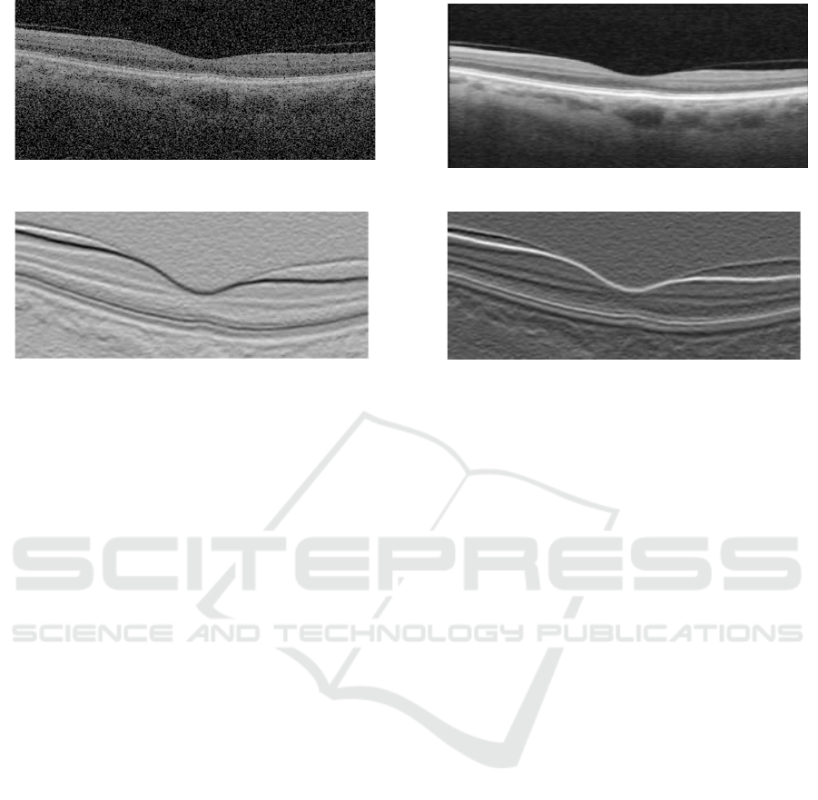
Figure 2: Image pre-processing. (a) Original image corrupted with speckle noise, and (b) ﬁltered image by Gaussian.

Figure 3: Image gradients used in generating (a) dark-bright adjacency matrix and (b) bright-dark adjacency matrix.

weights (w

min

), to enable the cut move freely in those

columns. This is based on the understanding that

each layer extends from the ﬁrst to last column of

the image, i.e. dividing the image horizontally at

each layer boundary, and that the Graph-Cut method

prefers paths with minimum weights. We use Djik-

stra’s algorithm (Dijkstra, 1959) in ﬁnding the min-

imum weighted path in the adjacency matrix (other

optimization methods utilizing sparse adjacency ma-

trices might be used in ﬁnding the minimum path).

Graph-Cut methods are optimal at ﬁnding one bound-

ary at a time, and therefore to segment multiple re-

gions in most cases, requires an iterative search in

limited space. Limiting the region of search is a com-

plex task, it requires prior knowledge and is depen-

dent on the structure of the features or regions of

interest. Some additional information on automatic

layer initialization and region limitation are discussed

in (Chiu et al., 2010) and (Kaba et al., 2015).

3.3 ILM and IS-OS Segmentation

It is commonly accepted that the NFL, IS-OS and

RPE exhibits high reﬂectivity in an OCT image (Chiu

et al., 2010; Lu et al., 2011; Tian et al., 2015).

Taking into account this reﬂectivity and the dark-

bright adjacency matrix we segment the ILM and IS-

OS boundaries using Dijkstras algorithm (Dijkstra,

1959). The ILM (vitreous-NFL) boundary is seg-

mented by searching for the highest change from dark

to light, this is because there is a sharp change in

the transition, additionally it is amidst extraneous fea-

tures, above it is the background region in addition to

no interruption of the blood vessels, as can be seen

in the gradient image. All of the above reasons make

it easier to segment the ILM than other layers. We

then limit the region below ILM and search for the

next highest change from dark-bright in order to seg-

ment the IS-OS boundary. In most cases the ILM is

segmented, but to account for uncertainties, i.e to dif-

ferentiate or conﬁrm which layer was segmented, we

use the mean value of the vertical axis of the paths to

determine the layer segmented, as the ILM is above

the IS-OS (similar to (Chiu et al., 2010).

3.4 RPE and NFL-GCL Segmentation

As mentioned in the previous subsection, RPE is one

of the most reﬂective layers. Using the bright-dark ad-

jacency matrix, the RPE-Choroid boundary exhibits

the highest bright-dark layer transition as can be seen

in Fig.3(a). Additionally based on experimental re-

sults, it is better to search for the transition from bright

to dark for the RPE, due to the interference of blood

vessels and the disruption of hyper-reﬂective pixels

in the choroid region. Therefore searching for the

bright-dark transition is ideal for the RPE most es-

pecially to adapt to noisy images. To segment the

NFL-GCL boundary,we limit the search space be-

tween ILM to IS-OS, and utilize the bright-dark ad-

jacency matrix to ﬁnd the minimum weighted path.

The resulting path is the NFL-GCL boundary, as it

is one of the most hyper-reﬂective layers. Addition-

ally if we limit our search space to regions below the

ILM and above the RPE, the resulting bright-dark and

dark-bright minimum paths are the NFL-GCL and IS-

OS respectively (i.e the NFL-GCL and IS-OS bound-

aries exhibits the second highest bright-dark and dark-

BIOIMAGING 2018 - 5th International Conference on Bioimaging

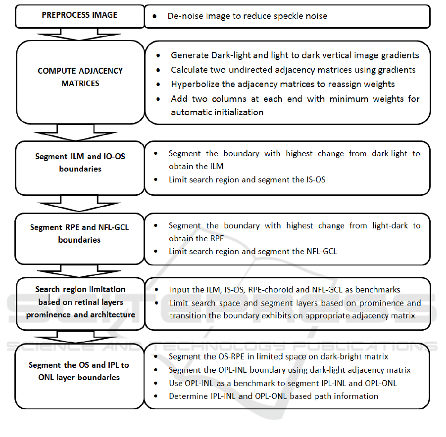
Figure 4: Main steps of segmentation algorithm schematic representation.

bright transition respectively in an OCT image).

3.5 OS and IPL to ONL Segmentation

To segment the OS-RPE and three other boundaries

(IPL-INL, INL-OPL, and OPL-ONL) from IPL to

ONL, we use the prior segmented layers as bench-

marks for search space limitation. We obtain the OS-

RPE region by searching for the dark-bright short-

est path between IS-OS and the RPE-Choroid. For

the remaining boundaries, ﬁrst we segment the INL-

OPL, because it exhibits a different transition among

the three. This is done by searching for the short-

est path between NFL-GCL and IS-OS on the dark-

bright adjacency matrix. Consequently the IPL-INL

and OPL-ONL boundaries are obtained by limiting

the region of path search between INL-OPL and NFL-

GCL, and INL-OPL and IS-OS regions respectively,

on the bright-dark adjacency matrix.

4 EXPERIMENTAL RESULTS

We evaluated the performance of the proposed

method on a set of 150 B-scan OCT images centred

on the macular region. This data set was collected

in Tongren Hospital with a standard imaging protocol

for retinal diseases such as glaucoma. The resolution

of the B-scan images are 512 pixels in depth and 992

pixels across section with 16 bits per pixel. We man-

ually labelled all the retinal layers in the dataset under

the supervision of clinical experts. This serves as the

Graph-Cut Segmentation of Retinal Layers from OCT Images

ground truth in our experiments. Prior to segment-

ing the images, 15% percent of the image height was

cropped from the top to remove regions with low sig-

nal and no features of interest. We segment seven reti-

nal layers automatically using MATLAB 2016a soft-

ware. The average computation time was 4.25 sec-

onds per image on a PC with Intel i5-4590 CPU, clock

of 3.3GHz, and 8GB RAM memory.

The method obtains the boundaries in the or-

der from ILM(Vitreous-NFL), IS-OS, RPE-Choroid,

NFL-GCL, OS-RPE, INL-OPL, IPL-INL to OPL-

ONL respectively. The locations of these boundaries

and the sequential order of the segmentation is shown

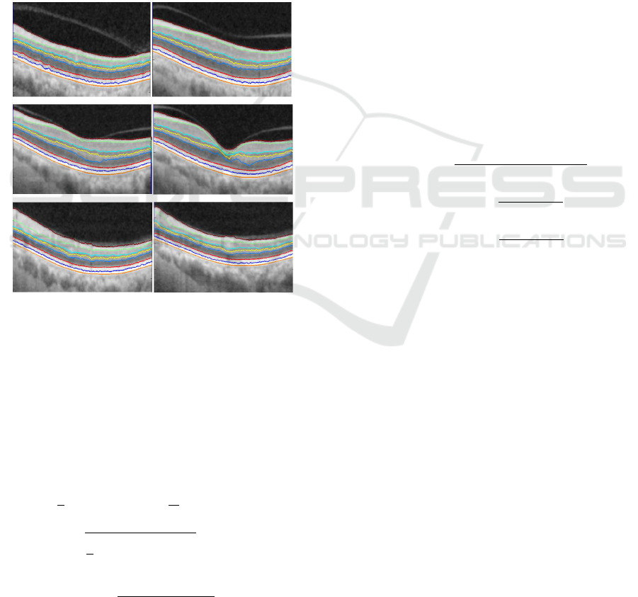
in Fig. 1. Sample results of the 8 retinal layer bound-

aries and the underlying 7 layers are shown in Fig. 5.

Figure 5: Segmentation results of 8 boundaries and 7 lay-

ers. Boundaries from top to bottom, the segmented bound-

aries are ILM, NFL-GCL, IPL-INL,INL-OPL, OPL-ONL,

IS-OS, OS-RPE and RPE-Choroid.

To evaluate the proposed method we calculate the

Root Mean Squared Error (RMSE), and Mean Abso-

lute Deviation (MAD) by (7). Table 1 shows the mean

and standard deviation of both MAD and RMSE, for

the seven layers targeted in this study.

MAD(GT, SEG) =

0.5 ∗

∑

i=1

d(pt

, SEG) +

∑

i=1

d(ps

, GT )

RMSE =

∑

i=1

(SEG

− GT

)

Dice =

2 | GT

∩ SEG

| GT

| + | SEG

(7)

where SEG

is the pixel labelled as retinal Layer by

the proposed segmentation method and GT

is the true

retinal layers pixel in the manually annotated image

(ground truth) image. pt

and ps

represent the coordi-

nates of the images, while d(pt

, SEG) is the distance

of pt

to the closest pixel on SEG with the same seg-

mentation label, and d(ps

, GT ) is the distance of ps

to the closest pixel on GT with the same segmenta-

tion label. n and m are the number of points on SEG

and GT respectively. For all layers our method has

performed well. Especially considering the low value

of NFL for both MAD and RMSE. The high value

in ONL+IS is due to the presence of high noise and

lower reﬂectivity of the boundaries within the region,

however, this is still considerably low.

Furthermore, We evaluated the retinal nerve ﬁ-

bre layer thickness (RNFLT) (the area between ILM

and NFL-GCL) with additional criteria, due to its

high importance in the diagnosis of ocular dis-

eases, including glaucoma. This is evaluated with

four criteria, namely, accuracy, sensitivity(true pos-

itive rate(TPR)), error rate(FPR) and the Dice in-

dex(coefﬁcient). These measurements are computed

with the following equations while the Dice is com-

puted from (8):

Accuracy =

T P + T N

(T P + FP + FN + T N)

Sensitivity(T PR) =

T P

(T P + FN)

ErrorRate(FPR) =

(FP + T N)

(8)

where T P, T N, FP and FN refers to true positive,

true negative, false positive and false negative respec-

tively. T P represents the number of pixels which are

part of the region that are labeled correctly by both

the method and the ground truth. T N represents the

number of pixels which are part of the background

region and labeled correctly by both the method and

the ground truth. FP represents the number of pixels

labeled as a part of the region by the method but la-

beled as a part of the background by the ground truth.

Finally, FN represents the number of pixels labeled

as a part of the background by the system but labeled

as a part of the region in ground truth. The results of

applying the above criteria on the RNFLT are shown

in Table 2.

5 CONCLUSIONS

We have presented an automatic segmentation method

for retinal OCT images that is capable of segment-

ing 7 retinal layers with 8 boundaries. The core of

BIOIMAGING 2018 - 5th International Conference on Bioimaging

Table 1: Performance evaluation with mean and standard deviation of RMSE and MAD for 7 retinal boundaries. 150 SD-OCT

B-Scan images (Units in pixels).

RetinalLayer MeanMAD MeanRMSE ST DMAD ST DRMSE

NFL 0.2689 0.0168 0.0189 0.0121

GCL+IPL 0.5938 0.0432 0.0592 0.0382

INL 0.6519 0.0387 0.0792 0.0612

OPL 0.5101 0.0446 0.0410 0.0335

ONL+IS 0.6896 0.0597 0.0865 0.0329

OS 0.4617 0.0341 0.0360 0.0150

RPE 0.4617 0.0341 0.0360 0.0150

Table 2: Mean accuracy, sensitivity, error rate, Dice and

Root Mean Squared Error (RMSE) of the Retinal Nerve

Fibre Layer Thickness (RNFLT) and standard deviation

(STD).

Measure ST D

Mean Accuracy 0.9816 0.0375

Mean Sensitivity 0.9687 0.0473

Mean Error Rate 0.0669 0.0768

Mean Dice 0.9746 0.0559

the method is a Graph-Cut segmentation using Dijk-

stra’s algorithm (Dijkstra, 1959). More importantly,

the adjacency matrices from vertical gradients and a

sequential process of segmentation, as two key ele-

ments of the study, are integrated into the Graph-Cut

framework. We have applied the proposed method to

a dataset of 150 OCT B-scan images, with successful

segmentation results. Further quantitative evaluation

indicates that the segmentation measurement is very

close to the ground-truth.

The main contributions of this work are as fol-

lows:

1. We have presented a method to automatically

identify 7 retinal layers across 8 layer boundaries,

so far one of the most comprehensive studies in

this area;

2. The adjacency matrices are effectively integrated

into the Graph-Cut framework with better weight

calculation;

3. Based on the unique characteristics of reﬂectivity

of different retinal layers and their changes across

layers, a sequential process of segmentation has

been developed.

REFERENCES

Baglietto, S., Kepiro, I. E., Hilgen, G., Sernagor, E.,

Murino, V., and Sona, D. (2017). Segmentation of

retinal ganglion cells from ﬂuorescent microscopy

imaging. In Proceedings of the 10th International

Joint Conference on Biomedical Engineering Systems

and Technologies (BIOSTEC 2017), pages 17–23.

Baroni, M., Fortunato, P., and La Torre, A. (2007). Towards

quantitative analysis of retinal features in optical co-

herence tomography. Medical engineering & physics,

29(4):432–441.

Boyer, K. L., Herzog, A., and Roberts, C. (2006). Auto-

matic recovery of the optic nervehead geometry in op-

tical coherence tomography. IEEE Transactions on

Medical Imaging, 25(5):553–570.

Boykov, Y. and Jolly, M.-P. (2001). Interactive Graph Cuts

for Optimal Boundary & Region Segmentation of Ob-

jects in N-D Images. Proceedings Eighth IEEE Inter-

national Conference on Computer Vision. ICCV 2001,

1(July):105–112.

Cabrera Fern

andez, D., Salinas, H. M., and Puliaﬁto, C. A.

(2005). Automated detection of retinal layer structures

on optical coherence tomography images. Optics Ex-

press, 13(25):10200.

Chiu, S. J., Li, X. T., Nicholas, P., Toth, C. a., Izatt, J. a., and

Farsiu, S. (2010). Automatic segmentation of seven

retinal layers in SDOCT images congruent with expert

manual segmentation. Optics express, 18(18):19413–

19428.

Dijkstra, E. W. (1959). A note on two problems in connex-

ion with graphs. Numerische mathematik, 1(1):269–

271.

Dodo, B., Li, Y., and Liu, X. (2017). Retinal oct image seg-

mentation using fuzzy histogram hyperbolization and

continuous max-ﬂow. In IEEE International Sympo-

sium on Computer-Based Medical Systems.

Ford, L. R. and Fulkerson, D. R. (1956). Maximal

ﬂow through a network. Journal canadien de

math

ematiques, 8:399–404.

Garvin, M. K., Abr

amoff, M. D., Wu, X., Russell, S. R.,

Burns, T. L., and Sonka, M. (2009). Automated 3-

D intraretinal layer segmentation of macular spectral-

domain optical coherence tomography images. IEEE

transactions on medical imaging, 28(9):1436–1447.

Haeker, M., Wu, X., Abr

amoff, M., Kardon, R., and Sonka,

M. (2007). Incorporation of regional information

in optimal 3-D graph search with application for in-

traretinal layer segmentation of optical coherence to-

mography images. Information processing in medical

Graph-Cut Segmentation of Retinal Layers from OCT Images

imaging : proceedings of the ... conference, 20:607–

618.

Huang, D., Swanson, E. A., Lin, C. P., Schuman, J. S.,

Stinson, W. G., Chang, W., Hee, M. R., Flotte, T.,

Gregory, K., and Puliaﬁto, C. A. (1991). Optical

coherence tomography. Science (New York, N.Y.),

254(5035):1178–81.

Kaba, D., Wang, Y., Wang, C., Liu, X., Zhu, H., Salazar-

Gonzalez, a. G., and Li, Y. (2015). Retina layer

segmentation using kernel graph cuts and continuous

max-ﬂow. Optics express, 23(6):7366–84.

Kolmogorov, V. and Zabih, R. (2004). What Energy Func-

tions Can Be Minimized via Graph Cuts? IEEE Trans-

actions on Pattern Analysis and Machine Intelligence,

26(2):147–159.

Koozekanani, D., Boyer, K., and Roberts, C. (2001). Reti-

nal thickness measurements from optical coherence

tomography using a Markov boundary model. IEEE

Transactions on Medical Imaging, 20(9):900–916.

Lang, A., Carass, A., Hauser, M., Sotirchos, E. S., Cal-

abresi, P. a., Ying, H. S., and Prince, J. L. (2013).

Retinal layer segmentation of macular OCT images

using boundary classiﬁcation. Biomedical optics ex-

press, 4(7):1133–52.

Lu, S., Yim-liu, C., Lim, J. H., Leung, C. K.-s., and Wong,

T. Y. (2011). Automated layer segmentation of op-

tical coherence tomography images. Proceedings -

2011 4th International Conference on Biomedical En-

gineering and Informatics, BMEI 2011, 1(10):142–

146.

Novosel, J., Vermeer, K. A., Thepass, G., Lemij, H. G., and

Vliet, L. J. V. (2013). Loosely Coupled Level Sets

For Retinal Layer Segmentation In Optical Coherence

Tomography. IEEE 10th International Symposium on

Biomedical Imaging, pages 998–1001.

Salazar-Gonzalez, A., Kaba, D., Li, Y., and Liu, X. (2014).

Segmentation of the blood vessels and optic disk in

retinal images. IEEE journal of biomedical and health

informatics, 18(6):1874–1886.

Seheult, A., Greig, D., and Porteous;, B. (1989). Exact

Maximum A Posteriori Estimation For Binary Images.

Journal of the Royal Statistical Society, Vol. 51(No.

2):271 –279.

Tian, J., Varga, B., Somfai, G. M., Lee, W. H., Smiddy,

W. E., and DeBuc, D. C. (2015). Real-time automatic

segmentation of optical coherence tomography vol-

ume data of the macular region. PLoS ONE, 10(8):1–

20.

Tizhoosh, H. R., Krell, G., and Michaelis, B. (1997). Lo-

cally Adaptive Fuzzy Image Enhancement. In Inter-

national Conference on Computational Intelligence,

pages 272–276. Springer.

Wang, C., Kaba, D., and Li., Y. (2015a). Level set segmen-

tation of optic discs from retinal images. Journal of

Medical Systems, 4(3):213–220.

Wang, C., Wang, Y., Kaba, D., Wang, Z., Liu, X., and Li,

Y. (2015b). Automated Layer Segmentation of 3D

Macular Images Using Hybrid Methods. Image and

Graphics, 9217:614–628.

Wang, C., Wang, Y., and Li, Y. (2017). Automatic choroidal

layer segmentation using markov random ﬁeld and

level set method. IEEE journal of biomedical and

health informatics.

Yuan, J., Bae, E., Tai, X.-C., and Boykov, Y. (2010). A study

on continuous max- ﬂow and min-cut approaches.

2010 IEEE Conference, 7:2217–2224.

Zhang, T., Song, Z., Wang, X., Zheng, H., Jia, F., Wu, J.,

Li, G., and Hu, Q. (2015). Fast retinal layer segmenta-

tion of spectral domain optical coherence tomography

images. Journal of Biomedical Optics, 20(9):096014.

BIOIMAGING 2018 - 5th International Conference on Bioimaging