Semi-automatic CT Image Segmentation using Random Forests

Learned from Partial Annotations

Old

rich Kodym

and Michal

Span

Department of Computer Graphics and Multimedia, Brno University of Technology,

Bozetechova 2, 612 66, Brno, Czech Republic

3Dim Laboratory, s.r.o., Kamenice 34, 625 00, Brno, Czech Republic

Keywords:

Computed Tomography, Semi-automatic Segmentation, Random Forests, Graph-cut.

Abstract:

Human tissue segmentation is a critical step not only in the process of their visualization and diagnostics but

also for pre-operative planning and custom implants engineering. Manual segmentation of three-dimensional

data obtained through CT scanning is very time demanding task for clinical experts and therefore the auto-

mation of this process is required. Results of fully automatic approaches often lack the required precision in

cases of non-standard treatment, which is often the case when computer planning is important, and thus semi-

automatic approaches demanding a certain level of expert interaction are being designed. This work presents a

semi-automatic method of 3D segmentation applicable to arbitrary tissue that takes several manually annota-

ted slices as an input. These slices are used for training a random forest classiﬁers to predict the annotation for

the remaining part of the CT scan and ﬁnal segmentation is obtained using the graph-cut method. Precision of

the proposed method is evaluated on various CT datasets using fully expert-annotated segmentations of these

tissues. Dice coefﬁcient of overlap is 0.976±0.014 for hard tissue segmentation and 0.978 ± 0.008 for kidney

segmentation, achieving competitive results with other task-speciﬁc methods.

1 INTRODUCTION

Three-dimensional segmentation of hard tissues in

medical Computed Tomography (CT) is a ﬁrst step re-

quired not only for reliable 3D visualization for diag-

nostic purposes but also for precise presurgical plan-

ning of orthopedic surgeries (Jun and Choi, 2010;

Wu et al., 2014) or craniofacial surgery (Chim et al.,

2014; Parthasarathy, 2014). Recently, number of 3D-

printable patient-speciﬁc implants (Tetsworth et al.,

2017) has also started to grow. Since these applicati-

ons require very accurate anatomical models, the seg-

mentation is often performed by clinical experts slice-

by-slice. As this task is very time demanding and te-

dious considering the number of slices in CT data, the

automation of this process is highly desirable. Howe-

ver, obstacles such as low-contrast tissue boundaries

and scatter which are usually present in CT data make

the automatic segmentation very difﬁcult. Also, met-

hods need to be robust against various pathologies and

anatomical variability.

Although fully automatic approaches often yield

acceptable results in standard cases where the patient

anatomy doesn’t strongly deviate from the norm, the

aforementioned applications often require precision

in cases of abnormalities such as fractures, lesions

etc. where these automatic methods very often fail.

Semi-automatic approaches allow the user to intro-

duce a priori case-speciﬁc information regarding the

desired result of the segmentation and alter the result

after the automatic segmentation, in case adjustment

is needed.

In this paper, we propose a new semi-automatic

method of 3D segmentation of arbitrary tissue in

medical CT scans based on Graph-Cut method and

Random Forests. The method searches for glo-

bally optimal binary segmentation of the volumetric

data with respect to probability ﬁelds acquired from

Random Forest classiﬁers trained online on several

expert-annotated slices. This method yields satis-

factory results while using as few as two orthogonal

user-annotated input slices as shown in Figure 1, al-

lowing for segmentation of objects with various de-

formities or pathologies. Additionally, we introduce

a novel way of encoding the voxel-wise classiﬁcation

into both the region-term and boundary-term energies

of the graph-cut framework.

124

Kodym, O. and Špan

el, M.

Semi-automatic CT Image Segmentation using Random Forests Learned from Partial Annotations.

DOI: 10.5220/0006588801240131

In Proceedings of the 11th International Joint Conference on Biomedical Engineering Systems and Technologies (BIOSTEC 2018) - Volume 2: BIOIMAGING, pages 124-131

ISBN: 978-989-758-278-3

Figure 1: An example of using the method. Input CT data

and two orthogonal user-annotated input slices (left) and the

segmentation result (right).

2 RELATED WORK

A number of methods of 3D medical data segmen-

tation is available in the literature up to date. The

most simple methods are segmentation of hard tis-

sues using adaptive thresholding of acquired Houns-

ﬁeld units (HU), which was applied to segmentation

of long bones (Rathnayaka et al., 2011) as well as

cranial bones (Pakdel et al., 2012) and region gro-

wing (Xi et al., 2014). All these methods are often

used in medical research as well as practice for their

simplicity, user-friendliness and easy understanding

of the method so behavior of a method can easily

be predicted. However, these methods require opti-

mal setting of threshold values and even then they are

prone to failure in locations where object boundaries

are very thin and low-contrast, as is often the case in

CT data due to partial volume artifact.

The more sophisticated approaches based on

active contour models such as level-sets (Pinheiro and

Alves, 2015) are able to complete the segmented ob-

ject boundary in these low contrast areas by making

assumptions about smoothness and continuity of the

boundary, but also tend to fail in areas of low intensity

gradient and are strongly dependable on user initiali-

zation of the object shape.

Methods utilizing statistical shape models (Yo-

kota et al., 2013) or active shape models (He et al.,

2016) form another category of segmentation approa-

ches that include preliminary creation of model of the

segmented object based on a training dataset acquired

from previous examinations. Such model can then be

registered to the current patient data using manually

located landmarks (Virzi et al., 2017) or automatically

(Chen et al., 2010). Use of shape models however as-

sumes that enough training data of the object is avai-

lable to sufﬁciently cover the physiological variability

and it usually doesn’t anticipate notable deviations in

the patient data.

In recent years, graph-cut methods based on (Boy-

kov and Jolly, 2001) gained some popularity as the

method is able to reliably and efﬁciently ﬁnd glo-

bally optimal segmentation of the object. While these

methods often require multiple iterations of user in-

teraction to achieve acceptable results (Shim et al.,

2009), another of their advantage is that they can ea-

sily utilize additional information such as output of

specialized edge detector (Kr

cah et al., 2011) or shape

model (Keustermans et al., 2012).

Convolutional neural networks (Krizhevsky et al.,

2012) are currently one of the fastest developing met-

hods in area of image processing. With the advance-

ments in computational power and expansion of va-

rious image databases, they became the state of the

art in numerous areas such as semantic image seg-

mentation (Zheng et al., 2015) as well as volumetric

medical data segmentation (Prasoon et al., 2013). In

this area, however, the available datasets still lack the

sufﬁcient scale and therefore the applications usually

rely heavily on synthetic dataset augmentation (Mil-

letari et al., 2016; Ronneberger et al., 2015). This

comes at cost of reduced robustness similar to the

model-based methods.

Classiﬁcation random forests (Loh, 2011) is

an ensemble machine learning method which uses

random subsets of available training dataset to con-

struct a set of binary decision trees. Each of these

trees, given a vector of input data, then outputs his-

togram of class probabilities and ﬁnally either voting

or averaging strategy is used to extract the ﬁnal clas-

siﬁcation of the ensemble of trees. The method has

been widely used in computer vision in recent years.

While random forests have lately been outperformed

by other machine-learning approaches such as con-

volutional neural networks in some image classiﬁca-

tion and segmentation tasks, random forests usually

require a much smaller training dataset and shorter

training time.

In this paper, we show that random forests lear-

ned using a few user-annotated slices only, in matter

of minutes, can achieve classiﬁcation accuracy sufﬁ-

cient to provide local voxel-wise predictions of tissue

boundaries for ﬁnal segmentation step based on glo-

bal graph-cut optimization.

3 GRAPH-CUT SEGMENTATION

WITH VOXEL-WISE

PROBABILITIES FROM

RANDOM FOREST

CLASSIFICATION

The segmentation method proposed in this paper ﬁrst

requires the user to manually denote contour of the

Semi-automatic CT Image Segmentation using Random Forests Learned from Partial Annotations

125

object in several slices, for example 3 orthogonal sli-

ces through the middle of the data volume. Next,

three voxel-wise random forest classiﬁers are trained

on the user annotated slices. Applying these classi-

ﬁers to the whole data volume outputs the probabi-

lity for each voxel to be a part of the object, its inner

edge and its outer edge. These three probability ﬁelds

are then converted into a graph structure where mi-

nimum cut/maximum ﬂow algorithm is employed to

ﬁnd the optimal binary segmentation of the object and

its background while re-using the user-annotated sli-

ces as hard constraints.

3.1 Random Forest Classiﬁcation

We formulate the segmentation as a binary classiﬁca-

tion problem where each voxel is assigned probabili-

ties of belonging inside or outside the segmented ob-

ject based on HU values of its surrounding voxels. A

lot of work has been put into choosing image features

suitable as input into the methods based on random

forests in the available literature. Various features

such as ﬁrst- and second-order statistics of the patch

surrounding the voxel (Cuingnet et al., 2012), entropy

metrics and Gabor features (Mahapatra, 2014) and

Haar-like features (Larios et al., 2010) have been used

for various segmentation tasks. However, our results

show that using only the intensity values from a small

volume patch surrounding the voxel yields sufﬁcient

trade-off between the results and training complexity,

which is important for semi-automatic method.

As mentioned earlier, we train following three se-

parate random forest classiﬁers:

• Object detector trained using the user-annotated

input binary object mask as the training data.

• Outer edge detector trained using the difference

between the user-annotated mask and its corre-

sponding 2D binary dilatation as the training data.

• Inner edge detector trained using the difference

between the user-annotated mask and its corre-

sponding 2D binary erosion as the training data.

The examples of detector outputs are shown in Fi-

gure 2 (d). The reason for training three separate clas-

siﬁers is explained in the following chapter.

3.2 Global Segmentation Reﬁnement

using Graph-cut

In our method, graph-cut is used to reﬁne the lo-

cal outputs of random forest classiﬁers into a com-

pact three-dimensional binary object. In the origi-

nal work by (Boykov and Jolly, 2001), the region-

and boundary-term energies used to ﬁnd the opti-

mal boundary are conventionally derived from origi-

nal image data as follows:

(”ob j”) = −ln[Pr(I

|O)] (1)

(”bkg”) = −ln[Pr(I

|B)] (2)

{p,q}

= exp

−

− I

)

2σ

dist(p, q)

, (3)

where Pr(I

|O) and Pr(I

|B) are probability values

corresponding to the intensity value of voxels extrac-

ted from histogram of user-annotated areas of image,

and I

are intensity values of the voxels and σ

is variance of intensity in data volume. Graph-cut

then ﬁnds the optimal segmentation by minimizing

the region-term energy over every individual voxel

and boundary-term energy over every combination of

neighboring voxels (6-neighborhood in 3D space).

Intuitively, we can replace the histogram-derived

probabilities in region term with the more task-

speciﬁc output of object detecting random forest clas-

siﬁer from the previous step as it is deﬁned for every

individual voxel. The new region-term energy is then

deﬁned as

(”ob j”) = −ln[RF

ob j

(p)] (4)

(”bkg”) = −ln[1 −RF

ob j

(p)], (5)

where RF

ob j

(p) is output of random forest object clas-

siﬁer for voxel p.

When deﬁning the boundary-term energy for reﬁ-

ning the output of voxel-wise classiﬁer, most appro-

aches such as (Mahapatra, 2014) decide to keep the

intensity-derived energy values or simply replace the

intensity difference with the difference of classiﬁer

output. This, however, discards the ability of the clas-

siﬁer to decide whether the object-background boun-

dary is likely between two given voxels. While it is

not practical to train and then evaluate a random fo-

rest classiﬁer on each possible combination of neig-

hboring voxels, it is possible to train two voxel-wise

classiﬁers and then combine their outputs. Conside-

ring a pair of neighboring voxels p and q with cor-

responding inner edge detector outputs RF

(p) and

(q) and outer edge detector outputs RF

out

(p) and

out

(q), the probability that the object-background

boundary lies in between these voxels is:

edge

(p, q) = RF

(p) · RF

out

(q) + RF

out

(p) · RF

(q).

(6)

BIOIMAGING 2018 - 5th International Conference on Bioimaging

126

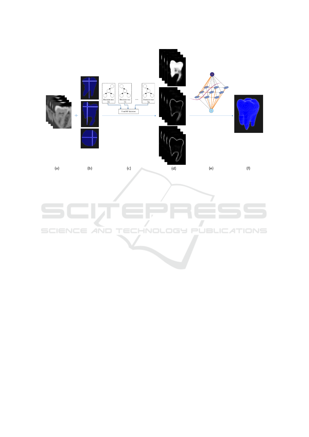
Figure 2: Overview of the segmentation framework. Original CT data (a) serve as an input along with several user-annotated

slices (b). Random forests (c) are then used to produce voxel-wise predictions of the object and its outer and inner edge (d).

These outputs are then integrated into a single graph structure (e) where min-cut/max-ﬂow algorithm is employed to ﬁnd ﬁnal

segmentation (f).

Therefore, we can deﬁne the new boundary-term

energy in following way:

{p,q}

= −ln[RF

(p) · RF

out

(q) + RF

out

(p) · RF

(q)].

(7)

While this approach is similar to (Browet et al.,

2016) who also add ”border” class to the classiﬁer be-

fore graph-cut, they derive the boundary-term energy

as maximum of the border penalization of the two

voxels while our method computes the penalization

for border between the two voxels speciﬁcally.

Similarly to the original method, we further use

the user-annotated slices as hard constraints by setting

the region-term energy of corresponding voxels to

(”ob j”) = 0 (8)

(”bkg”) = ∞ (9)

on voxels that user marked as object and to

(”ob j”) = ∞ (10)

(”bkg”) = 0 (11)

on the remaining voxels of the annotated slice. This

forces the ﬁnal segmentation to correspond to the

user’s initial shape description as the voxels already

annotated as the object can never be assigned back-

ground label and analogically the remaining voxels in

the slice can never have the object label. Finally, all

segmented objects not directly connected to any user-

deﬁned hard-constraints are discarded as false detecti-

ons.

4 EXPERIMENTS AND RESULTS

We conducted experiments on a medical CT data-

set that can be divided into three groups. The ﬁrst

group (A) consisted of 5 standard longitudinal bone

scans with 1.27 mm voxel spacing and 0.5 mm slice

thickness. These scans were fully manually segmen-

ted by medical expert and could therefore be used for

quantitative analysis of our method. The dataset in-

cluded three tibia, one humerus with higher level of

noise and one radial bone with higher level of blur.

Second group (B) consisted of two high-resolution

mandible scans. First scan with 0.4 mm voxel spa-

cing and 0.4 mm slice thickness included a toothless

mandible and had expert segmentation made in 11 ax-

ial slices. The second mandible with 0.3 mm voxel

spacing and 0.2 mm slice thickness had expert seg-

mentation made for individual teeth in 3 orthogonal

slices for each tooth. Scans in this group could not be

used for quantitative analysis due to lack of ground

truth and only illustrate that the method can be used

Semi-automatic CT Image Segmentation using Random Forests Learned from Partial Annotations

127

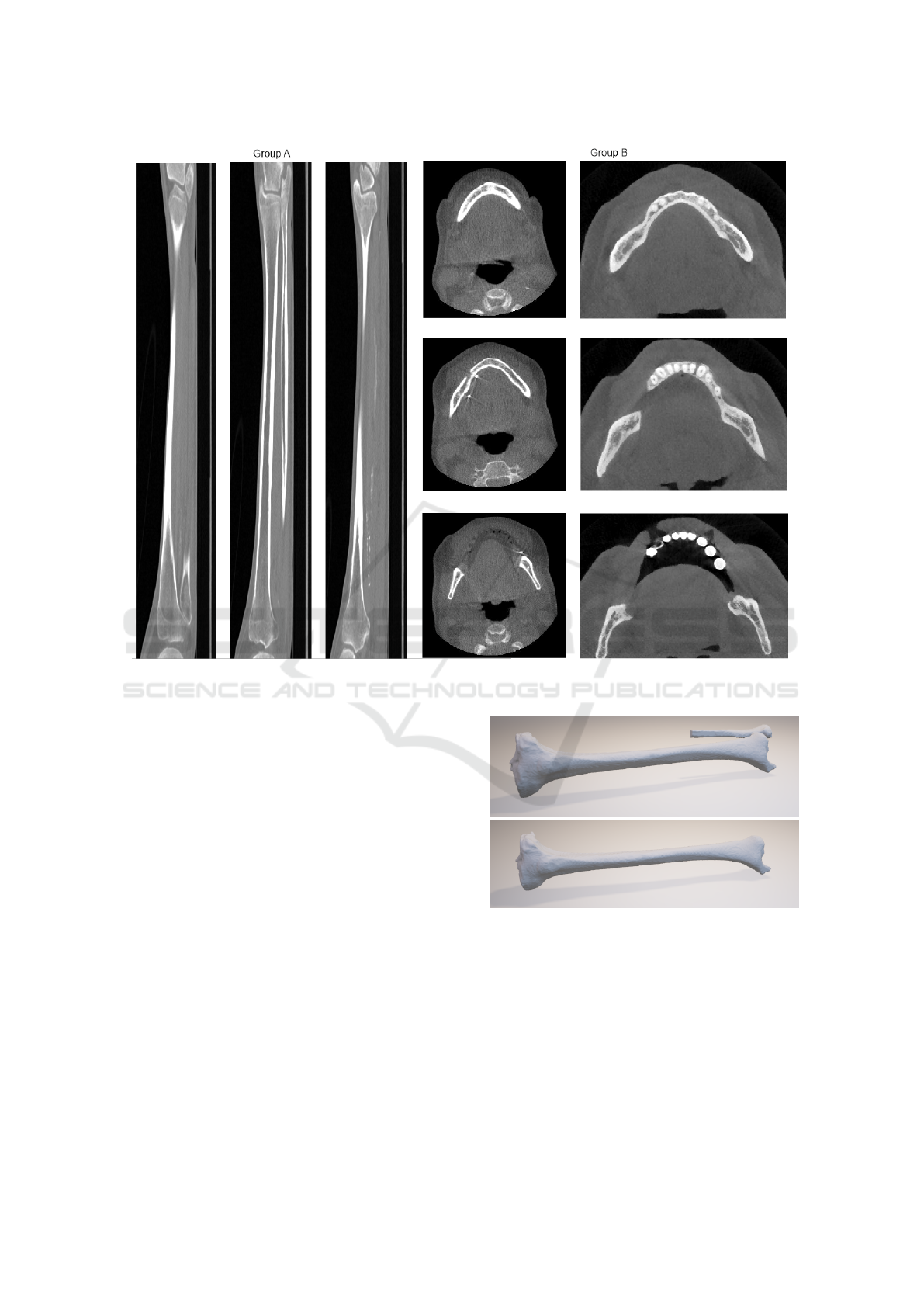
Figure 3: Example of CT scans on which the experiments were done. 3 lateral slices through a tibia in group A (left) and 3

axial slices of each mandible in group B (right).

to segment tissue of arbitrary shape. The third group

voxel spacing and 1.6 mm slice thickness. This da-

taset was also fully manually segmented to provide

ground truth. All scans were cropped around the ob-

jects of interest as an image pre-processing step. Ex-

amples of the scans in each group are shown in Fi-

gure 3.

The method was implemented in Python and Mat-

lab programming languages. Scikit-learn library

(Pedregosa et al., 2011) was used for implementa-

tion of the random forests and Visualization Toolkit

(Schroeder et al., ) for data vizualization. Matlab im-

plementation of the Maxﬂow algorithm (Boykov and

Kolmogorov, 2004) was used for the graph-cut opti-

mization. Tests were run on a laptop with 2.50GHz

i5-3210M processor and 8GB RAM. The required

computing time ranged from 4 minutes on smaller

data volumes such as single teeth scans to 15 minu-

tes on larger volumes such as shin bones.

For the scans in group A with full manual segmen-

tations available, Dice coefﬁcient (Dice, 1945) was

used to quantitatively determine accuracy of the pro-

Figure 4: Example of false negative segmentation of part of

splint-bone during shin-bone segmentation with Dice coef-

ﬁcient of 0.944 (upper) and correct shin-bone segmentation

after adding an additional input slice yielding Dice coefﬁ-

cient of 0.987 (lower).

posed method and to study dependency of its success

rate on the number of user-annotated slices used as

an input. The experiments showed a very high preci-

sion of the proposed method with Dice coefﬁcient of

0.976 ± 0.016 when using 5 user-annotated slices as

input, speciﬁcally 3 orthogonal slices through middle

BIOIMAGING 2018 - 5th International Conference on Bioimaging

128

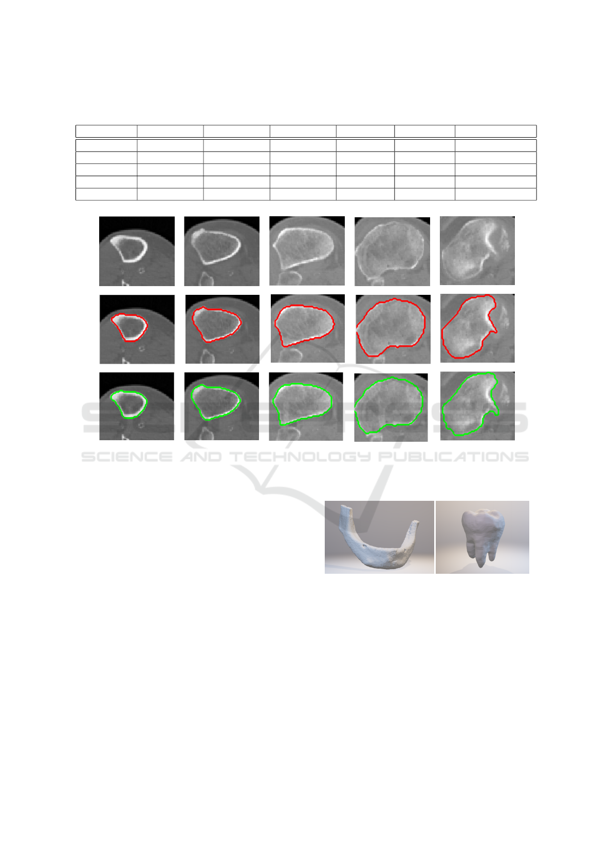
Table 1: Dice coefﬁcients (DC) of ﬁnal result and computation times of the classiﬁcation step of the method for individual

objects of interest. Training times for cases where 5 input slices were used are presented.

DC (2 slices) DC (3 slices) DC (5 slices) Total slices Training (s) Classiﬁcation (s)

Shin bone 1 0.983 0.983 0.984 770 95 423

Shin bone 2 0.959 0.968 0.991 530 182 764

Shin bone 3 0.944 0.944 0.987 540 134 386

Humerus 0.967 0.968 0.968 587 57 218

Radial bone 0.907 0.935 0.952 497 60 256

Figure 5: Example of result in 5 axial slices for the case where shin-bone was correctly segmented using only single frontal

and lateral slice as input. Red contour marks expert-annotated segmentation in these slices, green contour marks result of our

method.

of the bone and 2 additional axial slices through bone

proximities. When using more than 5 input slices, the

precision usually didn’t improve anymore. The spe-

ciﬁc results and computing times for each bone are

shown in Table 1. When using fewer user-annotated

slices, i.e. only one sagittal and one frontal slice, the

method still achieves high accuracy but can fail in se-

parating adjoining structures such as part of splint-

bone in case of shin-bone segmentation as shown in

Figure 4. This happens mostly when the adjoining

structure isn’t present in the annotated slices and can

be avoided by choosing the slices appropriately or by

allowing the user to interact with the graph-cut step of

the method. By marking only several voxels as being

false-positive detections, the graph-cut can be reeva-

luated in several seconds, incorporating the newly ad-

ded hard-constraints into the minimum cut search.

For the scans in group B, only several expert-

annotated slices were available and used as an input.

Although quantitative accuracy assessment is not pos-

Figure 6: Examples of the segmentation result for mandible

(left) and molar tooth (right). 11 axial slices were used as an

input for the mandible segmentation and 3 orthogonal slices

for the molar.

sible in these cases, the method yielded visually plau-

sible results in all cases when using the available user-

annotated slices as shown in Figure 6.

In experiments with the kidney scans in group

C, 3 orthogonal expert-annotated slices were used as

an input for each scan. The total number of ana-

lyzed slices per scan ranged from 59 to 83. The

mean Dice coefﬁcient of the segmentation results was

0.978 ± 0.008 achieving competitive results with ot-

Semi-automatic CT Image Segmentation using Random Forests Learned from Partial Annotations

129

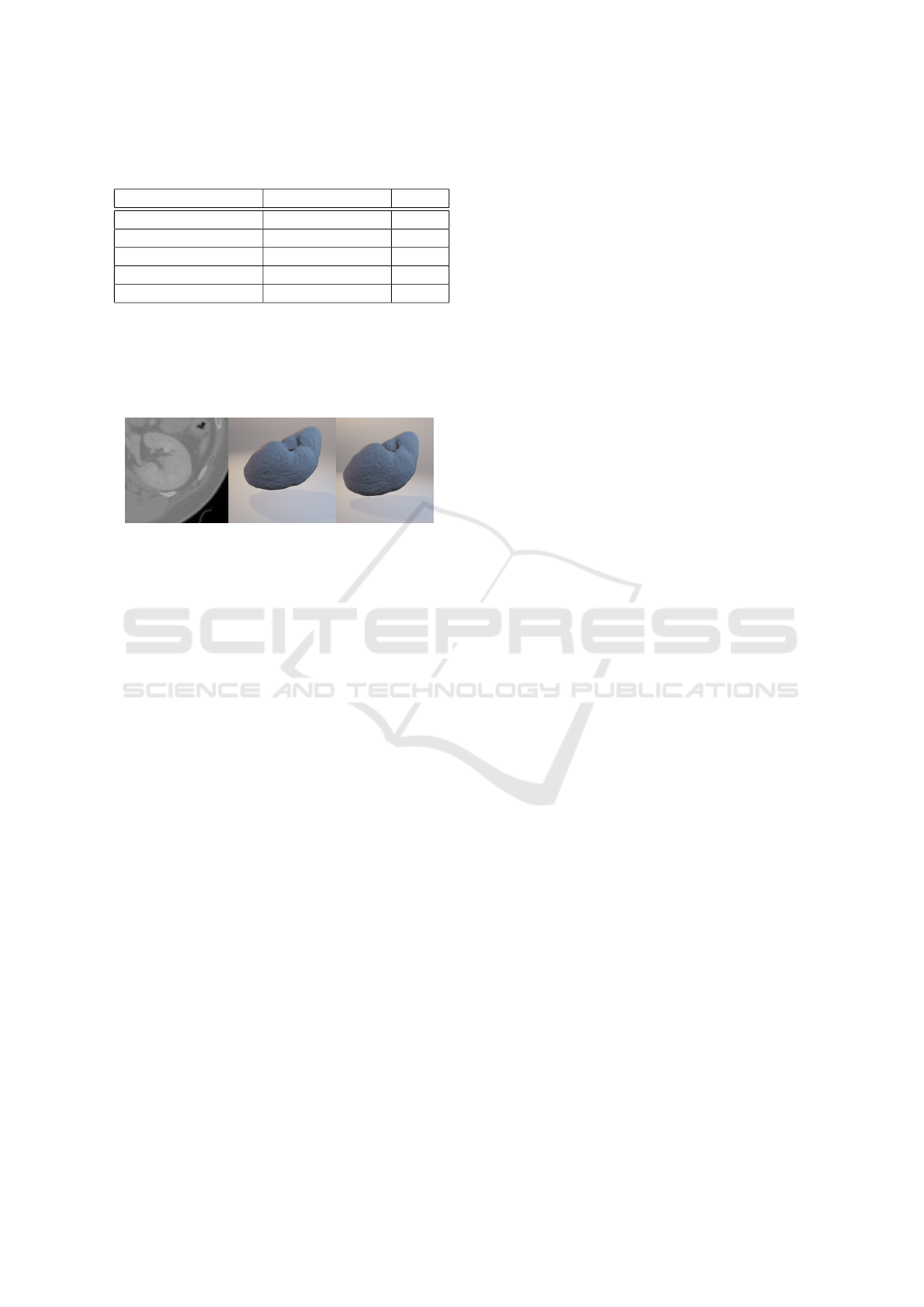
Table 2: Dice coefﬁcients (DC) of various kidney segmen-

tation methods.

Method Input DC

(Glisson et al., 2011) Seed points 0.93

(Sharma et al., 2015) 1 annotated slice <0.9*

(Sharma et al., 2017) None 0.86*

(Khalifa et al., 2017) None 0.97

Our method 3 annotated slices 0.98

* Results on CT scans of kidneys with autosomal dominant

polycystic kidney disease

her automatic and semi-automatic kidney segmenta-

tion methods as shown in Table 2. The example result

of segmentation by our method is shown in Figure 7.

Figure 7: Example of kidney segmentation. Original CT

data (left), manual segmentation (middle) and the output of

our method (right).

5 CONCLUSIONS

In this paper we proposed a method able to perform

segmentation of given tissue by ﬁrst interpolating

the user-annotated slices using random forest clas-

siﬁers and then reﬁning their output with graph-cut.

We also introduce a new methodology of incorpora-

ting an output of voxel-wise classiﬁer into boundary-

term energy of the graph structure generated from the

image in addition to the region-term energy.

The experiments show very good ﬁt of the results

with manually segmented tissues. After using hard

tissue dataset to tune and analyze the algorithm per-

formance, we tested it on the kidney dataset to show

that the output of our universal method is comparable

with state-of-the-art methods designed for the speciﬁc

task.

Although it takes more user input, i.e. several ma-

nually segmented 2D slices, when compared to other

methods, it brings signiﬁcant advantages. First, it al-

lows the user to segment an arbitrary tissue despite its

shape or intensity as the random forest classiﬁer infers

the appropriate object and edge features on its own as

long as the variability is captured in the annotated sli-

ces. Second, it is possible for the user to correct any

faulty segmented regions by including them in the an-

notated slices and then either reevaluating the graph-

cut optimization step in several seconds, or running

the full process again in case of larger errors. While

this takes several minutes for every iteration, it still sa-

ves a lot of time and manual work when correcting the

segmentation result in every slice individually. Also,

the computational complexity could be further redu-

ced by parallelizing the random forest classiﬁcation

step which takes majority of the computing time.

ACKNOWLEDGEMENTS

This work was supported in part by the company

3Dim Laboratory and by the Technology Agency of

the Czech Republic project TE01020415 (V3C - Vi-

sual Computing Competence Center). We would also

like to thank 3Dim Laboratory for providing us anno-

tated CT data for experiments.

REFERENCES

Boykov, Y. and Kolmogorov, V. (2004). An experimen-

tal comparison of min-cut/max- ﬂow algorithms for

energy minimization in vision. IEEE Transacti-

ons on Pattern Analysis and Machine Intelligence,

26(9):1124–1137.

Boykov, Y. Y. and Jolly, M.-P. (2001). Interactive Graph

Cuts for Optimal Boundary & Region Segmentation

of Objects in N-D Images.

Browet, A., Vleeschouwer, C., Jacques, L., Mathiah, N.,

Saykali, B., and Migeotte, I. (2016). Cell segmenta-

tion with random ferns and graph-cuts.

Chen, A., Deeley, M. A., Niermann, K. J., Moretti, L., and

Dawant, B. M. (2010). Combining registration and

active shape models for the automatic segmentation of

the lymph node regions in head and neck CT images.

Chim, H., Wetjen, N., and Mardini, S. (2014). Virtual surgi-

cal planning in craniofacial surgery. Seminars in Plas-

tic Surgery, 28(3):150–157.

Cuingnet, R., Prevost, R., Lesage, D., Cohen, L. D., Mory,

B., and Ardon, R. (2012). LNCS 7512 - Automa-

tic Detection and Segmentation of Kidneys in 3D CT

Images Using Random Forests.

Dice, L. R. . (1945). Measures of the Amount of Ecologic

Association Between Species. Ecology, 26(3):297–

302.

Glisson, C. L., Altamar, H. O., Herrell, S. D., Clark, P., and

Galloway, R. L. (2011). Comparison and assessment

of semi-automatic image segmentation in computed

tomography scans for image-guided kidney surgery.

Medical Physics, 38(11):6265–6274.

He, B., Huang, C., Sharp, G., Zhou, S., Hu, Q., Fang, C.,

Fan, Y., and Jia, F. (2016). Fast automatic 3D liver

segmentation based on a three-level AdaBoost-guided

active shape model. Medical Physics, 43(5):2421–

2434.

BIOIMAGING 2018 - 5th International Conference on Bioimaging

130

Jun, Y. and Choi, K. (2010). Design of patient-speciﬁc hip

implants based on the 3D geometry of the human fe-

mur. Advances in Engineering Software, 41(4):537–

547.

Keustermans, J., Vandermeulen, D., and Suetens, P. (2012).

Integrating Statistical Shape Models into a Graph Cut

Framework for Tooth Segmentation. pages 242–249.

Springer, Berlin, Heidelberg.

Khalifa, F., Soliman, A., Elmaghraby, A., Gimel’farb, G.,

and El-Baz, A. (2017). 3D Kidney Segmentation

from Abdominal Images Using Spatial-Appearance

Models. Computational and Mathematical Methods

in Medicine, 2017:1–10.

cah, M., Sz

ekely, G., and Blanc, R. (2011). Fully auto-

matic and fast segmentation of the femur bone from

3D-CT images with no shape prior. Proceedings - In-

ternational Symposium on Biomedical Imaging, pages

2087–2090.

Krizhevsky, A., Sutskever, I., and Hinton, G. E. (2012).

ImageNet Classiﬁcation with Deep Convolutional

Neural Networks.

Larios, N., Soran, B., Shapiro, L., Martinez-Munoz, G.,

Lin, J., and Dietterich, T. (2010). Haar Random Forest

Features and SVM Spatial Matching Kernel for Sto-

neﬂy Species Identiﬁcation. In 2010 20th Internatio-

nal Conference on Pattern Recognition, pages 2624–

2627. IEEE.

Loh, W.-Y. (2011). Classiﬁcation and regression trees.

Mahapatra, D. (2014). Analyzing Training Information

From Random Forests for Improved Image Segmen-

tation. IEEE Transactions on Image Processing,

23(4):1504–1512.

Milletari, F., Navab, N., and Ahmadi, S.-A. (2016). V-Net:

Fully Convolutional Neural Networks for Volumetric

Medical Image Segmentation. In 2016 Fourth Inter-

national Conference on 3D Vision (3DV), pages 565–

571. IEEE.

Pakdel, A., Robert, N., Fialkov, J., Maloul, A., and Whyne,

C. (2012). Generalized method for computation

of true thickness and x-ray intensity information in

highly blurred sub-millimeter bone features in clini-

cal CT images. Physics in Medicine and Biology,

57(23):8099–8116.

Parthasarathy, J. (2014). 3D modeling, custom implants and

its future perspectives in craniofacial surgery. Annals

of Maxillofacial Surgery, 4(1):9.

Pedregosa, F., Varoquaux, G., Gramfort, A., Michel, V.,

Thirion, B., Grisel, O., Blondel, M., Prettenhofer, P.,

Weiss, R., Dubourg, V., Vanderplas, J., Passos, A.,

Cournapeau, D., Brucher, M., Perrot, M., and Du-

chesnay, E. (2011). Scikit-learn: Machine learning

in Python. Journal of Machine Learning Research,

12:2825–2830.

Pinheiro, M. and Alves, J. L. (2015). A new level-set ba-

sed protocol for accurate bone segmentation from CT

imaging. IEEE Access, 3:1894–1906.

Prasoon, A., Petersen, K., Igel, C., Lauze, F., Dam, E., and

Nielsen, M. (2013). Deep Feature Learning for Knee

Cartilage Segmentation Using a Triplanar Convolutio-

nal Neural Network. pages 246–253. Springer, Berlin,

Heidelberg.

Rathnayaka, K., Sahama, T., Schuetz, M. A., and Schmutz,

B. (2011). Effects of CT image segmentation methods

on the accuracy of long bone 3D reconstructions. Me-

dical Engineering & Physics, 33(2):226–233.

Ronneberger, O., Fischer, P., and Brox, T. (2015). U-Net:

Convolutional Networks for Biomedical Image Seg-

mentation.

Schroeder, W. J., Martin, K. M., and Lorensen, W. E. The

Design and Implementation Of An Object-Oriented

Toolkit For 3D Graphics And Visualization.

Sharma, K., Peter, L., Rupprecht, C., Caroli, A., Wang, L.,

Remuzzi, A., Baust, M., and Navab, N. (2015). Semi-

Automatic Segmentation of Autosomal Dominant Po-

lycystic Kidneys using Random Forests.

Sharma, K., Rupprecht, C., Caroli, A., Aparicio, M. C., Re-

muzzi, A., Baust, M., and Navab, N. (2017). Auto-

matic Segmentation of Kidneys using Deep Learning

for Total Kidney Volume Quantiﬁcation in Autosomal

Dominant Polycystic Kidney Disease. Scientiﬁc Re-

ports, 7(1):2049.

Shim, H., Chang, S., Tao, C., Wang, J.-H., Kwoh, C. K., and

Bae, K. T. (2009). Knee Cartilage: Efﬁcient and Re-

producible Segmentation on High-Spatial-Resolution

MR Images with the Semiautomated Graph-Cut Algo-

rithm Method. Radiology, 251(2):548–556.

Tetsworth, K., Block, S., and Glatt, V. (2017). Putting 3D

modelling and 3D printing into practice: virtual sur-

gery and preoperative planning to reconstruct complex

post-traumatic skeletal deformities and defects. Sicot-

J, 3:16.

Virzi, A., Marret, J.-B., Muller, C., Berteloot, L., Boddaert,

N., Sarnacki, S., and Bloch, I. (2017). A new method

based on template registration and deformable models

for pelvic bones semi-automatic segmentation in pe-

diatric MRI. Proceedings - International Symposium

on Biomedical Imaging, pages 323–326.

Wu, D., Sofka, M., Birkbeck, N., and Zhou, S. K. (2014).

Segmentation of multiple knee bones from CT for ort-

hopedic knee surgery planning. Lecture Notes in Com-

puter Science (including subseries Lecture Notes in

Artiﬁcial Intelligence and Lecture Notes in Bioinfor-

matics), 8673 LNCS(PART 1):372–380.

Xi, T., Schreurs, R., Heerink, W. J., Berg

e, S. J., and

Maal, T. J. J. (2014). A novel region-growing ba-

sed semi-automatic segmentation protocol for three-

dimensional condylar reconstruction using cone beam

computed tomography (CBCT). PLoS ONE, 9(11):9–

14.

Yokota, F., Okada, T., Takao, M., Sugano, N., Tada, Y.,

Tomiyama, N., and Sato, Y. (2013). Automated CT

Segmentation of Diseased Hip Using Hierarchical and

Conditional Statistical Shape Models. pages 190–197.

Springer, Berlin, Heidelberg.

Zheng, S., Jayasumana, S., Romera-Paredes, B., Vineet, V.,

Su, Z., Du, D., Huang, C., and Torr, P. H. S. (2015).

Conditional Random Fields as Recurrent Neural Net-

works.

Semi-automatic CT Image Segmentation using Random Forests Learned from Partial Annotations

131