
Study of Route Optimization Considering Bottlenecks and Fairness
Among Partial Paths
Toshihiro Matsui
1
, Marius Silaghi
2
, Katsutoshi Hirayama
3
, Makoto Yokoo
4
and Hiroshi Matsuo
1
1
Nagoya Institute of Technology, Gokiso-cho Showa-ku Nagoya 466-8555, Japan
2
Florida Institute of Technology, Melbourne FL 32901, U.S.A.
3
Kobe University, 5-1-1 Fukaeminami-machi Higashinada-ku Kobe 658-0022, Japan
4
Kyushu University, 744 Motooka Nishi-ku Fukuoka 819-0395, Japan
Keywords:
Bottleneck, Fairness, Dynamic Programming, Search, A*, Route Optimization.
Abstract:
Route optimization is an important problem for single agents and multi-agent systems. In route optimization
tasks, the considered challenges generally belong to the family of shortest path problems. Such problems are
solved using optimization algorithms, such as the A* algorithm, which is based on tree search and dynamic
programming. In several practical cases, cost values should be as evenly minimized for individual parts of
paths as possible. These situations are also considered as multi-objective problems for partial paths. Since dy-
namic programming approaches are employed for the shortest path problems, different types of criteria which
can be decomposed with dynamic programming might be applied to the conventional solution methods. For
this class of problems, we employ a leximax-based criterion, which considers the bottlenecks and unfairness
among the cost values of partial paths. This criterion is based on a similar criterion called leximin for multi-
objective maximization problems. It is also generalized for objective vectors which have variable lengths.
We address an extension of the conventional A* search algorithm and investigate an issue concerning on-line
search algorithms. The influence of the proposed approach is experimentally evaluated.
1 INTRODUCTION
Route optimization is a critical problem for single
agents and multi-agent systems. Several tasks are
based on the optimization of routes, such as route
navigation for drivers, delivery services, and planning
for mobile robots. The goal of the route optimiza-
tion of agents is generally minimization of the total
cost on the optimal route. The A* search algorithm
is a fundamental path finding method that is based
on best-first search and dynamic programming (Hart
and Raphael, 1968; Hart and Raphael, 1972). On the
other hand, in several practical problems, improving
bottlenecks and fairness among the cost values of the
individual parts in the optimal path might be an is-
sue. This is also a multi-objective optimization prob-
lem where each objectivecorrespondsto an individual
part of a path. Several criteria, which select a solu-
tion to a multi-objective problem, are known as social
welfare or scalarization functions (Sen, 1997; Marler
and Arora, 2004). Leximin is a criterion that con-
siders bottlenecks and fairness among the objectives
for multi-objectivemaximization problems (Bouveret
and Lemaˆıtre, 2009; Greco and Scarcello, 2013). This
criterion is based on the dictionary order of vectors
whose values are sorted in ascending order. Maxi-
mization on the leximin criterion maximizes the min-
imum objective and improves fairness. This approach
has been applied to resource allocation problems with
multiple objectives (Dritan and Pioro, 2008). For the
minimization problems, similar a criterion where the
objective values are sorted in descending order can be
applied.
In this study, we focus on a property that a prob-
lem which is defined with this criterion can be decom-
posed into subproblems in ways similar to dynamic
programming (Matsui et al., 2014; Matsui et al.,
2015). Since the A* search algorithm is based on dy-
namic programming, we can employ a criterion that
resembles leximin. Therefore, in this work we ad-
dress the route optimization methods that improvethe
bottlenecks and the fairness of paths based on this
type of criterion. We apply a modified leximax cri-
terion that resembles leximin to the A* search algo-
rithm. We also investigate the possibility of incre-
mental optimization approaches for the exploration
Matsui, T., Silaghi, M., Hirayama, K., Yokoo, M. and Matsuo, H.
Study of Route Optimization Considering Bottlenecks and Fairness Among Partial Paths.
DOI: 10.5220/0006589000370047
In Proceedings of the 10th International Conference on Agents and Artificial Intelligence (ICAART 2018) - Volume 1, pages 37-47
ISBN: 978-989-758-275-2
Copyright © 2018 by SCITEPRESS – Science and Technology Publications, Lda. All rights reserved
37

1 2 3
4 5 6
7 8 9
1 1
1 1
1 1
1
211
22
Figure 1: Lattice graph.
of agents in environments. In this investigation, we
note that the proposed operations have a characteris-
tic property where the lower bounds of the optimal
path might not converge to the optimal values under
the equation of the optimal principle. On the other
hand, the upper bounds converge to the optimal ones.
We address how this property can be mitigated in in-
cremental optimization methods.
The rest of this paper is organized as follows.
The next section introduces the backgrounds of this
study, including path finding problems, related so-
lution methods, and several concepts about bottle-
necks and fairness. Then we present our proposed ap-
proach where a modified leximax criterion is applied
to the A* search algorithm in Section 3. Section 4
describes approaches for the exploration of agents in
environments. The proposed approach is experimen-
tally evaluated in Section 5. Then several discussions
and conclusions are shown in Sections 6 and 7.
2 PRELIMINARIES
2.1 Route Optimization Problems
Route optimization problems are generally based on
the shortest path problem. We address a fundamental
problem, which is defined with a weighted and undi-
rected graph G = hV, Ei. V and E are sets of ver-
tices and edges, respectively. We assume the edges
are undirected. For each edge e
i, j
∈ E, which is con-
nected to s
i
, s
j
∈ V, its cost value w
i, j
= ω(e
i, j
) is de-
fined with function ω : e
i, j
→ Z+, where Z+ is a set
of positive integer values.
Path P is defined as a sequence of vertices
(s
1
, s
2
, ··· , s
n
) ∈ V
n
, where edge e
i,i+1
∈ E exists be-
tween each pair of vertices s
i
, s
i+1
∈ V. The cost of
path P is evaluated as
∑
n−1
1
w
i, j
. The shortest path
from start node s
s
∈ V to goal node s
g
∈ V is defined
as the path with the minimum cost value among the
paths from s
s
to s
g
. Such a shortest path is considered
the optimal route.
In general settings, the aggregation of the cost val-
ues is defined with a summation operator to evaluate
the total summation of the cost values in a path. The
goal of the route optimization problem is to minimize
the cost of the routes for the same pair of start and
goal nodes.
In this work, we assume that the cost values take
a small number of integer values, such as {1, 2} or
{1, ··· , 10}. The cost values basically represent levels
of unfavorableness.
In the following, we interchangeably use vertices
and nodes. In addition, we mainly address lattice
graphs, as shown in Fig. 1, for simple discussions of
such issues as heuristic distances. Here, the numbers
of the nodes correspond to identifiers of them. The
numbers for the edges correspond to their cost values.
2.2 Path Finding Algorithm based on
Dynamic Programming
A* search (Hart and Raphael, 1968; Hart and
Raphael, 1972) is a path finding algorithm based on
best-first search and dynamic programming. This al-
gorithm performsa search process from a start node to
a goal node. In the process, the estimated cost values
(distances) of the optimal path are updated for the vis-
ited nodes by dynamic programming. When the goal
node is found, the optimal path is determined from
the stored information. In the exploration process, a
search method extends the nodes based on their esti-
mated cost values.
For each node s
i
∈ V, its estimated cost value of
optimal path f (s
i
) is defined:
f(s
i
) = g(s
i
) + h(s
i
). (1)
Here g(s
i
) is the estimated cost value from the start
node to s
i
, and h(s
i
) is the estimated cost value from
s
i
to the goal node. While g(s
i
) is updated based
on dynamic programming in the exploration process,
h(s
i
) is given as a heuristic value
1
. h(s
i
) is admis-
sible when it is a correct lower bound value. For
lattice graphs, h(s
i
) can be defined based on several
distance functions, such as the Manhattan and Euclid
distances, considering the lower bound cost values of
the edges.
The algorithm consists of two phases based on a
dynamic programming manner. In the first phase, an
optimal and complete version of best-first search is
performed from the start node s
s
updating each f(s
i
).
After the goal node s
g
is extracted, the second phase
is performed from the goal node to the start node to
compose the shortest path. See (Hart and Raphael,
1968; Hart and Raphael, 1972; Russell and Norvig,
2003) for details of the algorithm.
1
The actual algorithm maintains f(s
i
) as well as g(s
i
).
ICAART 2018 - 10th International Conference on Agents and Artificial Intelligence
38

2.3 Real-time Search Algorithm
Real-time search algorithms are also path finding
methods based on search methods and dynamic pro-
gramming. Here the solution methods are designed so
that an agent employs exploration and exploitation in
a path finding. Initially, the agent is placed at the start
node with estimated cost values (e.g. h(s
i
) = 0 for all
s
i
∈ V). It explores in the environment and learns the
estimated optimal cost value of each node. Based on
these estimated cost values, the agent searches for the
goal node. After the agent arrives at the goal node, it
starts its next tour with the updated values.
An important point of this approach is that dy-
namic programming is assumed to be the agent’s
learning process. With an appropriate strategy and
learning rule, the estimated optimal cost value of each
node is improved by the number of tours. Learning
Real-Time A* (LRTA*) is such an algorithm. With it,
an agent performs the following steps at each node s
i
in a tour:
1. For all nodes s
j
adjacent to s
i
, the agent evaluates
estimated cost value f(s
j
) = w
i, j
+ h(s
j
).
2. The agent updates the estimated cost value so that
h(s
i
) ← min
s
j
f(s
j
).
3. It moves to the next node so that s
i
←
arg min
s
j
f(s
j
).
Note that in the above rule, the h(s
i
) value is both
the estimation value to be optimized and the penalty
value that is employed to escape from cyclic paths.
See (Barto et al., 1995) for details of this algorithm.
2.4 Bottlenecks and Fairness Among
Edges
Next we investigate the improvement of bottlenecks
and fairness among edges. In the example in Fig. 1,
let the start node be s
s
= 1 and the goal node be s
g
= 9.
In the minimization of conventional total cost values,
one optimal path is (1, 2, 3, 6, 9) and its cost is 5. On
the other hand, for minimization where the edges of
the maximal cost values are reduced, one optimal path
is (1, 2, 3, 6, 5, 8, 9), and its cost is 6. Note that there
are no edges with cost value 2 on this path. Here the
goal of the problem is not only to reduce the number
of edges with the maximum cost values but also to
reduce the total cost value by improving the fairness
among edges, if possible. Such paths might be inves-
tigated when an appropriate route must avoid highly
unsatisfactory specific residents and extra loads of
bottleneck facilities.
2.5 Multi-objective Optimization
Problems
In the class of multi-objective optimization prob-
lems, multiple objectives are simultaneously opti-
mized. The above route optimization problem with
bottlenecks and fairness is also a multi-objective op-
timization problem. Here we consider the following
multi-objective optimization problem: MOP.
Definition 1 (MOP). MOP is defined with hX, D, Fi.
X is a set of variables, D is a set of domains of vari-
ables, and F is a set of objective functions. Variable
x
i
∈ X takes value from finite and discrete set D
i
∈ D.
For set of variables X
i
⊆ X, function f
i
∈ F is de-
fined as f
i
(x
i,1
, ··· , x
i,k
) : D
i,1
× ···× D
i,k
→ N, where
x
i,1
, ··· , x
i,k
∈ X
i
. f
i
(x
i,1
, ··· , x
i,k
) is simply denoted by
f
i
(X
i
). The goal of the problem is to simultaneously
optimize the objective functions under a criterion.
A combination of the values of the objective func-
tions is represented as an objective vector.
Definition 2 (Objective vector). Objective vector v
is defined as [v
1
, ··· , v
K
]. For assignment A to the
variables in X
j
, v
j
is defined as v
j
= f
j
(A
↓X
j
).
Here the ideal goal is to maximize all the values
of the objective functions. However, in general cases,
the goal cannot be achieved since there are trade-
offs between the objectives. Therefore, based on the
Pareto dominance between objective vectors, one of
the Pareto optimal solutions is selected (Sen, 1997;
Marler and Arora, 2004).
2.6 Leximin
Since there are many Pareto optimal solutions in gen-
eral cases, several social welfare criteria and scalar-
ization functions are employed to select a solu-
tion (Sen, 1997; Marler and Arora, 2004).
Summation
∑
K
j=1
f
j
(X
j
), which is found in con-
ventional social welfare, considers the efficiency of
the objectives. While maximization on the summation
achieves Pareto optimality, fairness among the objec-
tives is ignored. Maximin maximizes minimum objec-
tive value min
K
j=1
f
j
(X
j
). Even though this improves
the worst case value among the objectives, the solu-
tion is not Pareto optimal. To ensure Pareto optimal-
ity, such additional tiebreaker criteria as summation
are necessary. Moreover, since only the minimum ob-
jective value is improved, other objective values are
not distinguished.
Leximin is defined as the dictionary order on ob-
jective vectors whose values are sorted in ascending
order (Bouveret and Lemaˆıtre, 2009; Greco and Scar-
cello, 2013; Matsui et al., 2014; Matsui et al., 2015).
Study of Route Optimization Considering Bottlenecks and Fairness Among Partial Paths
39

Definition 3 (Sorted objective vector). The values of
sorted objective vector v are sorted in ascending or-
der.
Definition 4 (Leximin). Let v = [v
1
, ··· , v
K
] and v
′
=
[v
′
1
, ··· , v
′
K
] denote the sorted objective vectors whose
length is K. The order relation, denoted with ≺
leximin
,
is defined as follows. v ≺
leximin
v
′
if and only if
∃t, ∀t
′
< t, v
t
′
= v
′
t
′
∧ v
t
< v
′
t
.
Leximin is a criterion that repeats the comparison
between the minimum values in the vectors. Since
maximization on leximin is a subset of maximin, it
improves the worst case values. In addition, this max-
imization relatively improves the fairness and ensures
Pareto optimality.
The addition of two sorted objective vectors is de-
fined with concatenation and resorting.
Definition 5 (Addition of sorted objective vec-
tors). Let v and v
′
denote vectors [v
1
, ··· , v
K
] and
[v
′
1
, ··· , v
′
K
′
], respectively. The addition of two vectors,
v⊕ v
′
, is represented as v
′′
= [v
′′
1
, ···v
′′
K+K
′
], where v
′′
consists of all the values in v and v
′
. In addition, the
values in v
′′
are sorted in ascending order.
For the addition of sorted objective vectors, the
following invariance exists (Matsui et al., 2014).
Proposition 1 (Invariance of leximin on addition).
Let v and v
′
denote sorted objective vectors of the
same length. In addition, v
′′
denotes another sorted
objective vector. If v ≺
leximin
v
′
, then v ⊕ v
′′
≺
leximin
v
′
⊕ v
′′
.
Based on this invariance, dynamic programming
can be applied to solve optimization problems with
the leximin criterion (Matsui et al., 2014; Matsui
et al., 2015). However, we assume that the original
problem is decomposed into subproblems with objec-
tive vectors of the same length.
Moreover, a sorted objective vector can be repre-
sented as a vector of the sorted pairs of an objective
value and the count of the value (Matsui et al., 2014).
This representation corresponds to run-length encod-
ing and a sorted histogram. The comparison and the
addition of two sorted objective vectors can be di-
rectly performed on this representation.
2.7 Theil Index
As addressed above, several criteria, including sum-
mation and leximin, ensure Pareto optimality. Pareto
optimality is important in situations with selfish mem-
bers; however, other measurements of inequality are
also critical. To evaluate the paths shown in later sec-
tions, we employ the Theil index, a well-known mea-
surement of inequality.
Definition 6 (Theil Index). For n objectives, Theil in-
dex T is defined as
T =
1
n
∑
i
v
i
¯v
log
v
i
¯v
(2)
where v
i
is the utility or the cost value of an objective
and ¯v is the mean utility value for all the objectives.
The Theil index takes a value in [0, logn]. When
all utilities or cost values are identical, the Theil in-
dex value is zero. Inequalities on different number of
members can be compared using it. Note that the min-
imization on the leximin criterion does not assure the
decrement of the Theil index value, since it is basi-
cally a sequence of improvements of the worst value.
3 ROUTE OPTIMIZATION
CONSIDERING BOTTLENECKS
AND FAIRNESS
We address the route optimization problems that
consider bottlenecks and fairness among individual
edges. As shown in the previous section, the opti-
mization problem with the leximin criterion is decom-
posed with dynamic programming. Therefore, we in-
vestigate the approach that replaces the aggregation
of the cost values in the A* algorithm from the sum-
mation to a leximin-like criterion. Assuming the new
criterion for this optimization, the problem is rede-
fined as follows.
The shortest path finding problem is defined with
a weighted and undirected graph G = hV, Ei. The sets
V, E, weight values of edges, and Path P are defined
similar to the original definition. The cost of path
P is aggregated as a objective vector instead of the
summation. Then the cost is compared based on a
criterion which is similar to the leximin, while it is
designed for minimization problems and the variable
length of vectors. The shortest path from start node
s
s
∈ V to goal node s
g
∈ V is defined as the path with
the minimum cost value based on this criterion. Such
a shortest path is considered the optimal route.
The following two modifications must be ad-
dressed to employ the approach for maximization on
the leximin criterion.
• The maximization on leximin is replaced by the
minimization on leximax.
• The operations are extended for the subproblems
of different lengths of vectors.
ICAART 2018 - 10th International Conference on Agents and Artificial Intelligence
40

3.1 Minimization on Leximax
For minimization problems, maximization on leximin
is replaced by the minimization of leximax. Although
leximax is similarly defined as leximin, the ordering
of the values in the objective vectors is inverted.
Definition 7 (Descending sorted objective vector).
The values of a descending sorted objective vector are
sorted in descending order.
Definition 8 (Leximax). Let v = [v
1
, ··· , v
K
] and
v
′
= [v
′
1
, ··· , v
′
K
] denote descending objective vectors
whose lengths are K. The order relation, denoted with
≺
leximax
, is defined as follows. v ≺
leximax
v
′
if and only
if ∃t, ∀t
′
< t, v
t
′
= v
′
t
′
∧ v
t
< v
′
t
.
With this modification, the worst case values are
inverted to maximum cost values. Thus the objective
of the problem is also inverted to the minimization of
the aggregated objective values. While the addition of
two descending sorted objective vectors is similarly
defined as the leximin, the ordering of the values in
each concatenated vector is the opposite.
3.2 Comparison of Vectors with
Different Lengths
In route optimization problems, when the path lengths
are different, the lengths of the corresponding objec-
tive vectors are also different. Therefore, we employ
the variable-length leximax, vleximax, whose defi-
nition is extended for objective vectors of different
lengths.
Definition 9 (Vleximax). Let v = [v
1
, ··· , v
K
] and
v
′
= [v
′
1
, ··· , v
′
K
′
] denote descending sorted objective
vectors whose lengths are K and K
′
, respectively. For
K = K
′
, ≺
vleximax
is the same as ≺
leximax
. In other
cases, zero values are appended to one of the vectors
so that the both vectors have the same number of val-
ues. Then the vectors are comparedbased on ≺
leximax
.
Intuitively, this comparison is based on two modi-
fied vectors which have the same sufficient length by
padding blanks with zeros. Consider the two modified
vectors of infinite length assuming the cost of zero for
each unused edge, which can contain the extra edges
outside of the system. Since the comparison of lexi-
max is based on tie-breaks from the beginning of the
both vectors, the redundant parts of zeros in both the
vectors can be ignored.
In the A* search algorithm for comparing two
paths based on vleximax, the corresponding descend-
ing sorted objective vector should be appropriately
aggregated.
3.3 Heuristic Distance Function
In the A* search algorithm, estimated cost value h(v
i
),
which is given by a heuristic distance function, should
be a lower bound value that does not exceed the op-
timal cost value. For example, in the case of lattice
graphs, such a heuristic function can be defined with
the lower bound cost value for all the edges and the
Manhattan distance. For minimization on the summa-
tion, a heuristic value is the product of the Manhattan
distance and the lower bound cost value.
For minimization on the vleximax, such a heuris-
tic value is an objective vector that consists of dupli-
cates of the lower bound cost values, where the vector
length is identical to the Manhattan distance.
3.4 Correctness and Complexity of
Solution Method
When the objective vector of estimated cost h(v
i
) of
a heuristic distance function is a correct lower bound
one, the A* search algorithm selects one of the op-
timal paths. For lattice graphs, the Manhattan dis-
tance from a node to the goal node is the minimum
length of the possible vector. Therefore, the objec-
tive vector whose length is the same as the Manhattan
distance and whose values are duplicates of the low-
est cost value for all the edges is a lower bound for
the remaining optimal path. On the other hand, in
general cases, designing efficient heuristic functions
might not be easy.
In addition, for minimization on summation,
heuristic cost value h(v
i
) can be simply defined as
zero. Similarly, for minimization on leximax, an
empty vector can be employed as h(v
i
).
The comparison of two vectors of different lengths
based on vleximin activates a tiebreaker, where the
shorter vector is selected when the two vectors are
identical on their parts of the same length. In this case,
fewer edges are preferred. Since the estimation cost
is a lower bound, no incorrect path can be selected as
the optimal path, even if the lengths of the descending
sorted objective vectors are different. Therefore, the
solution method returns one of the optimal paths.
Even though the overhead of the computation re-
lated to vleximax is significantly larger than that of
the summation and the comparison on scalar val-
ues, it is polynomial with the length of each vector.
When the sorted objective vector is represented as
run-length encoding or a histogram, the space com-
plexity of each vector is O(n) for n types of objective
values. If an array is employed for this vector repre-
sentation, the addition of two vectors increments the
Study of Route Optimization Considering Bottlenecks and Fairness Among Partial Paths
41

1 2 3
4 5 6
7 8 9
1 2
1 1
1 1
1
111
22
Figure 2: Lattice graph with walls.
count values whose complexity is O(n). The com-
plexity for the comparison of two vectors is also O(n).
4 INCREMENTAL
OPTIMIZATION
Next we focus on how the real-time search algorithm
can be generalized with the leximax criterion. Un-
fortunately, this is impossible due to a problematical
monotonicity on cyclic paths.
Consider the case shown in Fig. 2, where the
agents start from node 1. For the nodes adjacent to
node 1, h(2) + w
1,2
= [ ] + [1] = [1] and h(4) + w
1,4
=
[ ] + [2] = [2]. With the vleximax and the rules based
on the LRTA* shown in Section 2.3, the agent moves
to node 2 and updates h(1) to [1]. Then for the nodes
adjacent to node 2, h(1) + w
1,2
= [1] + [1] = [1, 1],
h(3) + w
2,3
= [ ] + [2] = [2], and h(5) + w
2,5
= [ ] +
[2] = [2]. Therefore, the agent returns to node 1 and
updates h(2) to [1, 1]. In the third step, for the nodes
adjacent to node 1, h(2)+ w
1,2
= [1, 1] +[1] = [1, 1, 1]
and h(4) + w
1,4
= [ ] + [2] = [2]. Therefore, the agent
returns to node 2 again and repeats this round-trip for-
ever to add cost value 1 to h(1) and h(2).
The above example reveals the necessity of other
approaches for exploration in the case of sorted ob-
jective vectors with variable lengths when there can
be cyclic paths. Such cyclic paths can be detected
with a threshold length. Then some such incorrect
vectors can be replaced by appropriate vectors that
break the cyclic movements. However, such an ap-
proach might be problematic, since the invariance of
vleximin does not hold and may affect the correctness
of the dynamic programming.
4.1 Episode-based Approach
Here we address more safe approaches with a rela-
tively direct extension of conventional search algo-
rithms. Since the dynamic programming is correct,
we employ episode-based learning, where the learn-
ing phases are separated from the exploration phase.
This approach is also called off-line learning.
Assume that a complete path between the start and
goal nodes was obtained from an exploration phase.
Cyclic paths are allowed to increase the learning op-
portunities.
Then the path is scanned from the goal node to the
initial start node by updating corresponding estimated
values h(s
k
) except the goal node. Note that here s
k
denotes the k
th
value from the initial start node on a
path:
1. The agent evaluates f(s
k+1
) = w
i, j
+ h(s
k+1
),
where w
i, j
corresponds to edge e
i, j
between s
k
and
s
k+1
.
2. If h(s
k
) has not been updated yet, it is up-
dated by f(s
k+1
). Otherwise, it is updated by
min( f(s
k+1
), h(s
k
)).
In the example of Fig. 2, assume that an episode
of nodes (1, 2, 3, 6, 5, 2, 3, 6, 9) has been performed in
the initial trial. Since the node 9 is the goal node,
h(9) holds empty vector []. Then h(6) is updated by
f(9) = [] + [1] = [1]. Similarly, for their previous part
of nodes (5, 2, 3), h(3) = [1, 1], h(2) = [1, 1, 2], h(5) =
[1, 1, 2, 2] are updated. However, for their previous
node 6, h(6) holds its vector by min( f(5), h(6)) =
min([1, 1, 1, 2, 2], [1]) = [1]. h(3) = [1, 1] and h(2) =
[1, 1, 2] are also unchanged for the previous part of
nodes (3, 2). Finally, h(1) is updated by [1, 1, 1, 2].
The above h(s
k
) is the upper bound of the optimal
cost value from s
k
to the goal node, since it is up-
dated by the propagation from the goal node. When
the agent’s explorations are sufficient, h(s
k
) converges
to the optimal value, since the algorithm exactly per-
forms partial updates of the dynamic programming.
4.2 Boundaries of Paths
While the above episode-based approach needs com-
plete paths to the goal nodes, it converges with ap-
propriate exploration strategies. The other problem of
the above simple update rule is that it does not employ
the information of neighborhood nodes which are not
on the path. Also, the algorithm cannot evaluate the
lower bound cost values which can be employed by
best-first strategies.
Here we address the lower bound of optimal cost
value h
(s
i
) and the upper bound value h(s
i
). The
boundaries h
(s
i
) and h(s
i
) of the estimated cost val-
ues are initialized as follows:
1. Except for the goal node, h
(s
i
) and h(s
i
) are ini-
tialized to [ ] and [⊤···⊤], respectively, where ⊤
denotes the maximum cost value. h(s
i
) must con-
tain a sufficient number of duplicates of the maxi-
mum cost value to exceed the other objective vec-
tors in the manner of vleximin.
ICAART 2018 - 10th International Conference on Agents and Artificial Intelligence
42

2. On the other hand, for the goal node, the initial
value of h(s
i
) and h(s
i
) is [ ].
Except for the goal node, node s
i
updates its h
(s
i
)
and h(s
i
) as follows:
h(s
i
) ← max(h(s
i
), min
s
j
(w
i, j
+ h(s
j
))) (3)
h(s
i
) ← min(h(s
i
), min
s
j
(w
i, j
+ h(s
i
))), (4)
where s
j
denotes all the nodes adjacent to s
i
. Here we
update h
(s
i
) and h(s
i
) at the same time.
When a path is obtained from an exploration
phase, the following operations are performed.
1. The path is scanned from the goal node to the first
node.
2. Except for the goal node, each node s
i
on the path
updates its h
(s
i
) and h(s
i
).
With the above boundaries the exploration and
learning phases perform parts of dynamic program-
ming. We consider that the boundaries of node s
i
have
converged when h
(s
i
) ≥ h(s
i
). In the case of the con-
ventional summation, the boundaries eventually con-
verge. However, in the case of the vleximax, the con-
vergence is not guaranteed. Consider the example
shown in Fig. 2 again. Assuming that h
(3), h(4), and
h
(5) take zero, from the initial state, h(1) and h(2)
increase such that [ ], [1], [1, 1], [1, 1, 1], ··· , [1, · · · , 1]
by turns. These vectors never overcome a vector
[2]. Similar cases occur in actual propagations even
if an episode does not contain cyclic paths. For a non
cyclic path (1, 2, 3, 6, 9), the lower bounds are updated
for the sequence of nodes 1 and 2 in reverse order.
If other paths of different episodes contain these two
nodes, they are repeatedly updated in a way that is
similar to the above manner.
This situation resembles LRTA* which is not eas-
ily generalized with vleximax. In this problem, the
upper bounds of cost vectors still follow the principle
of optimality. On the other hand, the lower bounds
might not converge to the optimal vectors, while their
lengths monotonically increase. This property also
resembles that of negative cyclic paths. The A* al-
gorithm dose not affected by this property, since it is
based on the propagation of cost values from the node
of zero cost. In addition, the algorithm does not as-
sume cyclic paths. However, LRTA* is affected by
the property, since its behavior is completely based
on the lower bounds. Therefore, the on-line search
might be caught by cyclic paths.
To mitigate such situations, we revise the cor-
rupted lower bound as follows.
1. When the length of h
(s
i
) exceeds the number of
edges, h
(s
i
) is replaced by f (s
j
) which is the sec-
ond smallest value: f
(s
j
) = secondmin
s
k
(w
i,k
+
h(s
k
)). If such all values are corrupted, it means
that there is no information to fix the boundaries.
Therefore, the agent do nothing and wait for fu-
ture propagations from outside.
2. This modification may cause the situation of
h
(s
i
) 6≤ h(s
i
) as a result of propagations. In this
case, h
(s
i
) is replaced by h(s
i
).
This approach is not exact but based on the im-
mediate convergence of upper bounds. Since we em-
ploy an off-line learning which updates both upper
and lower bounds simultaneously from the node of
zero cost (i.e. the goal node), the convergence of up-
per bounds will be faster than the lower bounds in
general cases. In addition, the revision of a broken
lower bound vector is performed when its length ex-
ceeds a threshold. It also delays the convergence of
the lower bounds. When these assumptions are suf-
ficiently satisfied, it is expected that the solution will
resemble the one of A*.
4.3 A Heuristic Exploration
The exploration strategies should cover all solutions
with boundaries. Even though arbitrary exploration
strategies can be employed, we employ a heuristic ex-
ploration strategy as follows. We added the following
information to each node s
i
.
• the counter vstcnt
i
of visits to the node in each
tour. The counter is reset to zero in the beginning
of each exploration process.
• the last visit time lasttime
i
to the node. This infor-
mation is stored through the optimization process.
We employ a logical time which is incremented
after it is stored to a lastime
i
. In the initial state,
all lasttime
i
are set to zero.
Similarly, the following information is added to
each edge.
• the counter selcnt
i, j
of selection of the edge e
i, j
in each tour. The counter is reset to zero in the
beginning of each exploration process.
With the above information, the following rules
are applied to an agent on s
i
adjacent to nodes s
j
.
1. If s
j
is the goal node, s
j
has the first priority.
2. For s
j
and an edge e
i, j
, if h
(s
j
) 6= h(s
j
) and
selcnt
i, j
= 0, s
j
has the second priority. This rule
assures to evaluate unexplored edges even if those
cost values are relatively high.
3. The node s
j
who has a smaller vstcnt
i
has the third
priority. With this rule, the agent will avoid cyclic
paths if possible.
Study of Route Optimization Considering Bottlenecks and Fairness Among Partial Paths
43

Table 1: Solution qualities: lattice graph of 10× 10 nodes.
Cost Alg. Solution quality
sum. min. max. len. theil
[1, 2] sum. 20.7 1 2 18 0.039
lxm. 21.9 1 2 19.6 0.032
[1, 5] sum. 34.3 1 4 18 0.135
lxm. 41.3 1 3.4 22.4 0.095
[1, 10] sum. 58.6 1 7.7 18.4 0.223
lxm. 74.4 1 6.6 23.2 0.147
Table 2: Solution qualities: Lattice graph of 100 × 100
nodes.
Cost Alg. Solution quality
sum. min. max. len. theil
[1, 2] sum. 213.2 1 2 198 0.025
lxm. 286.9 1 2 282.8 0.006
[1, 5] sum. 346.1 1 5 199.6 0.132
lxm. 446.7 1 3.6 275.6 0.085
[1, 10] sum. 580.8 1 9.5 202.8 0.215
lxm. 960.3 1 6.8 350 0.128
Table 3: Computational cost: lattice graph of 100 × 100
nodes.
cost alg. iter. num. of exec.
opn. nodes time [s]
[1, 2] sum. 7217 7537 0.022
lxm. 8359 8883 0.070
[1, 5] sum. 9989 9996 0.020
lxm. 9497 9923 0.078
[1, 10] sum. 9996 9999 0.019
lxm. 8468 9182 0.172
4. When vstcnt
i
are identical, the node s
j
who has
a lower h(s
j
) has the fourth priority. This is the
best-first strategy, which is guided by the above
rules.
5. When vstcnt
i
and h
(s
j
) are are identical, respec-
tively, then the node s
j
with older lasttime
i
has
the fifth priority. With this rule, ties will be ex-
plored deterministically.
Due to the above boundaries and the heuristic ex-
ploration, the resulting solution method might be an
inexact method; however they fit particular intuitions
based on our experience. As the first study, we experi-
mentally employ the aboveapproach assuming simple
graphs. The necessity of such a guided approach for
the vleximax criterion reveals the difficulty of design-
ing an on-line optimization algorithm for this class of
problems.
Table 4: Solution qualities: lattice graph of 10 × 10 nodes
(start nodes in the middle).
cost alg. solution quality
sum. min. max. len. theil
[1, 2] sum. 11.8 1 2 10 0.045
lxm. 12.5 1 1.8 11 0.037
[1, 5] sum. 20 1 3.7 10 0.133
lxm. 26.4 1 3.4 14.2 0.096
[1, 10] sum. 34.5 1.2 7.1 10.4 0.199
lxm. 50.6 1.1 6.3 15.4 0.134
Table 5: Solution qualities: Lattice graph of 100 × 100
nodes (start nodes in the middle).
cost alg. solution quality
sum. min. max. len. theil
[1, 2] sum. 108.5 1 2 100 0.027
lxm. 149.5 1 1.8 147 0.006
[1, 5] sum. 178.5 1 4.9 100.8 0.132
lxm. 223.2 1 3.4 135 0.087
[1, 10] sum. 301 1 9 103.2 0.213
lxm. 592.1 1 6.3 214.8 0.130
Table 6: Computational cost: lattice graph of 100 × 100
nodes (start nodes in the middle).
cost alg. iter. num. of exec.
opn. nodes time [s]
[1, 2] sum. 1993 2182 0.004
lxm. 7013 7371 0.066
[1, 5] sum. 4702 4860 0.009
lxm. 9214 9702 0.105
[1, 10] sum. 7023 7217 0.016
lxm. 7759 8402 0.175
5 EVALUATION
We experimentally evaluated the proposed approach.
First, we evaluated the modified A* search algorithm.
The example problems are based on lattice graphs that
consist of 10 × 10 and 100 × 100 nodes. Start node
s
s
and goal node s
g
are the left-top and right-bottom
nodes. Each edge has an integer cost value in [1, 2],
[1, 5], or [1, 10]. The cost value is randomly set based
on uniform distribution. Ten problem instances are
averaged for each set of parameters. We experimen-
tally compared the conventional method based on the
summation ‘sum.’ and the proposed method based
on leximax (vleximax) ‘lxm.’. The experiment was
performed on a computer with a Core i7-3930K CPU
(3.20 GHz), 16-GB memory, Linux 2.6.32, and g++
(GCC) 4.4.7.
Tables 1 and 2 show the solution qualities. The
cost values in each solution are evaluated with the
summation, the minimum value, the maximum value,
ICAART 2018 - 10th International Conference on Agents and Artificial Intelligence
44
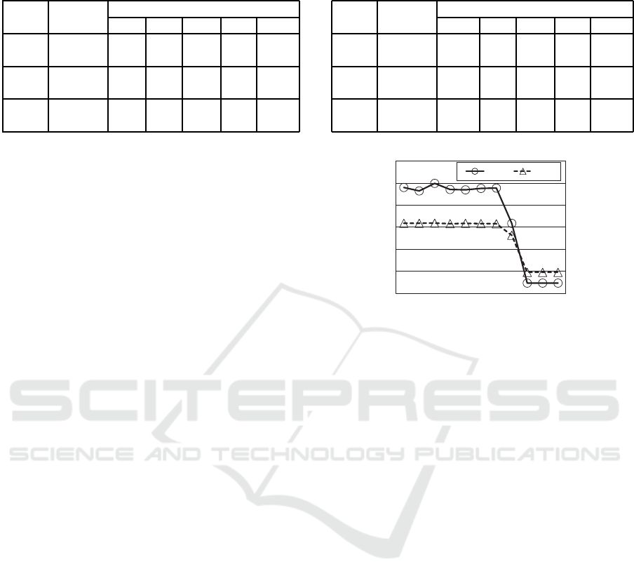
Table 7: Solution qualities: lattice graph of 10× 10 nodes
(lxm) (A* and learning).
cost alg. solution quality
sum. min. max. len. theil
[1, 2] lxm. A* 21.9 1 2 19.6 0.032
lxm. lrn. 21.9 1 2 19.6 0.032
[1, 5] lxm. A* 41.3 1 3.4 22.4 0.095
lxm. lrn. 41.3 1 3.4 22.4 0.095
[1, 10] lxm. A* 74.4 1 6.6 23.2 0.147
lxm. lrn. 74.4 1 6.6 23.2 0.147
the number of values (len.), and the Theil index
(theil). The Theil index is a criterion of unfairness,
where smaller values represent less unfairness. The
results show that the solution method ‘lxm.’ reduced
bottlenecks and unfairness with trade-offs between
them and the summation. It also reduced the Theil in-
dex on average. In addition, the maximum cost value
was reduced whenever possible.
Table 3 shows the computational cost. We eval-
uated the computational cost as the number of oper-
ations for the nodes (iter.), the number of extended
nodes (num. of opn. nodes), and the execution
time. The result reveals that the heuristic cost func-
tion based on the Manhattan distance on the grids is
not very efficient. While most of the nodes were ex-
tended, there were several opportunities for pruning,
even for the solution method ‘lxm.’ The execution
time of ‘lxm.’ significantly exceeded that of ‘sum.’
due to the operations on the sorted objective vectors
and vleximax. But overhead might be allowed in rel-
atively small problems.
With the same set of graphs, we evaluated the
cases where a start node s
s
is almost in the center of
a graph, while a goal node is the right-bottom node.
Tables 4 and 5 show the solution qualities. The results
resemble the cases of the previous setting. Similarly,
Table 6 shows the computational cost. In this result,
the number of extracted nodes is relatively less than
that of the previous setting. It is considered as the
effect of the heuristic distance function of the A* al-
gorithm. On the other hand, the reduction for ‘lxm.’
is relatively small. This reveals the difficulty of de-
signing heuristic distance functions for the criterion.
We also evaluated the optimization methods for
the exploration agents. Here 10 × 10 and 20 × 20
lattice graphs with left-top start nodes s
s
and right-
bottom goal nodes s
g
are employed. The A* algo-
rithm based on vleximax (‘lxm. A*’) and the incre-
mental solution method (‘lxm. lrn.’) were evaluated.
With preliminary experiments, we set appropriate pa-
rameters so that the incremental solution method ob-
tains episodes and the solution quality converges. Ta-
Table 8: Solution qualities: lattice graph of 20 × 20 nodes
(lxm) (A* and learning).
cost alg. solution quality
sum. min. max. len. theil
[1, 2] lxm. A* 46.8 1 1.9 44.8 0.016
lxm. lrn. 46.8 1 1.9 44.8 0.016
[1, 5] lxm. A* 77.4 1 3.4 45.4 0.102
lxm. lrn. 77.4 1 3.4 45.4 0.102
[1, 10] lxm. A* 145.7 1 6.6 50.6 0.145
lxm. lrn. 145.7 1 6.6 50.6 0.145
0
0.05
0.1
0
100
200
300
400
500
600
100 300 500 700 900 1100
theil
sum.
trial
sum theil
Figure 3: Incremental optimization with vleximax: 20× 20
nodes, w
i, j
= [1, 2].
bles 7 and 8 shows the solution quality. Since both
methods obtain similar results, it is considered that
the heuristic approaches of the incremental solution
method are relatively reasonable.
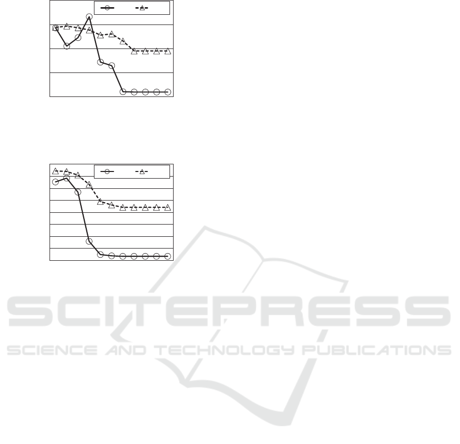
Figures 3-5 show the learning progress of the in-
cremental solution methods. Each graph shows the
anytime curves of the summation and the Theil in-
dex for an actual result. The samples are averaged
for every 100 trials. Note that the results can vary
for instances, since we employed a relatively exhaus-
tive exploration based on best-first search. The results
show that the summation and the Theil index were
gradually improved and converged. In addition, the
Theil index was relatively small in early trials when
the range of cost values was also narrow.
6 DISCUSSION
Since maximization on (v)leximax improves the
worst case values, the summation of the cost values
is increased as a trade-off. When the range of the
cost values is relatively large, the trade-off is empha-
sized, and hence the increment of the summation of
the cost values grows. The length of the optimal vec-
tor, namely the number of edges in the optima path,
also grows. Additional approaches, such as limita-
tions on the ranges of the cost values or controls of
Study of Route Optimization Considering Bottlenecks and Fairness Among Partial Paths
45
0
0.05
0.1
0.15
0.2
0
500
1000
1500
2000
100 300 500 700 900 1100
theil
sum.
trial
sum theil
Figure 4: Incremental optimization with vleximax: 20× 20
nodes, w
i, j
= [1, 5].
0
0.05
0.1
0.15
0.2
0
500
1000
1500
2000
2500
3000
3500
4000
100 300 500 700 900 1100
theil
sum.
trial
sum theil
Figure 5: Incremental optimization with vleximax: 20× 20
nodes, w
i, j
= [1, 10].
criteria, are necessary to reduce the trade-offs. On the
other hand, the proposed method’s solution can pro-
vide an analysis based on a criterion that addressed
bottlenecks and fairness.
In this work, we assumed lattice graphs and em-
ployed a distance function based on the Manhattan
distance, which relays the possible minimum length
of the vectors. For other topologies of the graphs and
more efficient estimations, additional considerations
are necessary.
In general, most criteria that strictly address fair-
ness cannot be easily decomposed into parts based on
dynamic programming. In this study, we focused on
how leximin/leximax-based criteria can be applied to
dynamic programming methodsfor path finding prob-
lems. Even though the aggregation and the compari-
son of the criteria can almost be directly applied, the
exploration process needs other methods to avoid in-
correct results due to the problematical monotonicity
of lower bound vectors on cyclic paths.
In addition, leximin/leximax is different from
summation in several aspects. For example, when the
two neighboring edges are aggregated into an edge,
the resulting edge can be related to the aggregation of
the two original cost values. While the resulting cost
value is still a scalar value for the summation, a vec-
tor of two values is necessary to maintain the original
information for the leximin/leximax. Such general-
ization needs more investigation.
Since this criterion is simply defined without pa-
rameters, the trade-offs among bottleneck, fairness
and effectiveness are fixed. Several modifications or
different criteria that can be decomposed with dy-
namic programming will be necessary to maintain the
trade-offs.
7 CONCLUSION
We addressed route optimization methods that con-
sider bottlenecks and fairness on optimal paths using
maximization on leximax criteria. The experimental
results shows that our proposed approach reduced the
cases of the worst cost values and relatively improved
the fairness in the optimal path. Future work will
improve the solution methods including better heuris-
tic functions and investigations about similar criteria
with more appropriate tunings of trade-offs between
efficiency and fairness. The opportunities of on-line
learning and reinforcement learning will also be inter-
esting issues.
ACKNOWLEDGEMENTS
This work was supported in part by JSPS KAKENHI
Grant Number JP16K00301.
REFERENCES
Barto, A. G., Bradtke, S. J., and Singh, S. P. (1995). Learn-
ing to act using real-time dynamic programming. Ar-
tificial Intelligence, 72(1-2):81–138.
Bouveret, S. and Lemaˆıtre, M. (2009). Computing leximin-
optimal solutions in constraint networks. Artificial In-
telligence, 173(2):343–364.
Dritan, N. and Pioro, M. (2008). Max-min fairness and its
applications to routing and load-balancing in commu-
nication networks - a tutorial. IEEE Communications
Surveys and Tutorials, 10(4):5–17.
Greco, G. and Scarcello, F. (2013). Constraint satisfac-
tion and fair multi-objective optimization problems:
Foundations, complexity, and islands of tractability.
In Proc. 23rd International Joint Conference on Arti-
ficial Intelligence, pages 545–551.
Hart, P., N. N. and Raphael, B. (1968). A formal basis
for the heuristic determination of minimum cost paths.
IEEE Trans. Syst. Science and Cybernetics, 4(2):100–
107.
ICAART 2018 - 10th International Conference on Agents and Artificial Intelligence
46

Hart, P., N. N. and Raphael, B. (1972). Correction to ’a for-
mal basis for the heuristic determination of minimum-
cost paths’. SIGART Newsletter, (37):28–29.
Marler, R. T. and Arora, J. S. (2004). Survey of
multi-objective optimization methods for engineer-
ing. Structural and Multidisciplinary Optimization,
26:369–395.
Matsui, T., Silaghi, M., Hirayama, K., Yokoo, M., and Mat-
suo, H. (2014). Leximin multiple objective optimiza-
tion for preferences of agents. In 17th International
Conference on Principles and Practice of Multi-Agent
Systems, pages 423–438.
Matsui, T., Silaghi, M., Okimoto, T., Hirayama, K., Yokoo,
M., and Matsuo, H. (2015). Leximin asymmetric mul-
tiple objective DCOP on factor graph. In 18th In-
ternational Conference on Principles and Practice of
Multi-Agent Systems, pages 134–151.
Russell, S. and Norvig, P. (2003). Artificial Intelligence: A
Modern Approach (2nd Edition). Prentice Hall.
Sen, A. K. (1997). Choice, Welfare and Measurement. Har-
vard University Press.
Study of Route Optimization Considering Bottlenecks and Fairness Among Partial Paths
47
