Road Boundary Detection using In-vehicle Monocular Camera

Kazuki Goro and Kazunori Onoguchi

Graduate School of Science and Technology, Hirosaki University, 3 Bunkyo-cho, Hirosaki, 036-8561, Japan

Keywords:

Inverse Perspective Mapping, ITS, Shoulder of a Road, Snow Wall, Snakes.

Abstract:

When a lane marker such as a white line is not drawn on the road or it’s hidden by snow, it’s important for

the lateral motion control of the vehicle to detect the boundary line between the road and the roadside object

such as curbs, grasses, side walls and so on. Especially, when the road is covered with snow, it’s necessary to

detect the boundary between the snow side wall and the road because other roadside objects are occluded by

snow. In this paper, we proposes the novel method to detect the shoulder line of a road including the boundary

with the snow side wall from an image of an in-vehicle monocular camera. Vertical lines on an object whose

height is different from a road surface are projected onto slanting lines when an input image is mapped to a

road surface by the inverse perspective mapping. The proposed method detects a road boundary using this

characteristic. In order to cope with the snow surface where various textures appear, we introduce the degree

of road boundary that responds strongly at the boundary with the area where slant edges are dense. Since the

shape of the snow wall is complicated, the boundary line is extracted by the Snakes using the degree of road

boundary as image forces. Experimental results using the KITTI dataset and our own dataset including snow

road show the effectiveness of the proposed method.

1 INTRODUCTION

For the past several decades, many vision-based lane

detection methods have been proposed for advanced

driver assistance system or autonomous driving sys-

tem(M. Bertozzi, A. Broggi, M. Cellario, A. Fas-

cioli, P. Lombardi and M. Porta, 2002)(J. C. Mc-

Call and M. M. Trivedi, 2006)(B. Hillel, R. Lerner,

D. Levi, and G. Raz, 2014). Most of these meth-

ods detect lane markers such as white lines from an

image and estimate a trafﬁc lane. In the literature

(M. Bertozzi and A. Broggi, 1998), a belt-like re-

gion whose width is constant and whose brightness

is higher than a road surface is detected as a lane

marker. In the literature (J.Douret, R. Labayrade, J.

Laneurit and R. Chapuis, 2005), a lane marker is de-

tected from a pair of the positive edge and the nega-

tive edge with constant distance. The literature (M.

Meuter, S. Muller-Schneiders, A. Mika, S. Hold, C.

Numm and A. Kummert, 2009) proposes the method

that detects a boundary of the white line from a peak

of the histogram of edge gradient. The literature (C.

Kreucher and S. Lakshmanan, 1999) proposes the

method that detects a lane marker by extracting a

slanting edge by DCT. The method to detect a broken

line(S. Hold, S. Gormer, A. Kummert, M. Meuter, S.

Muller-Schneiders, 2010) or a zebra line(G. Thomas,

N. Jerome and S. Laurent, 2010) by a frequency anal-

ysis is also proposed. The literature (Z. W. Kim,

2008) detects a lane marker by a discriminator cre-

ated by learning many lane marker images.

Although these methods are effective for roads on

which lane markers are drawn, they can not be ap-

plied to roads without lane markers or roads covered

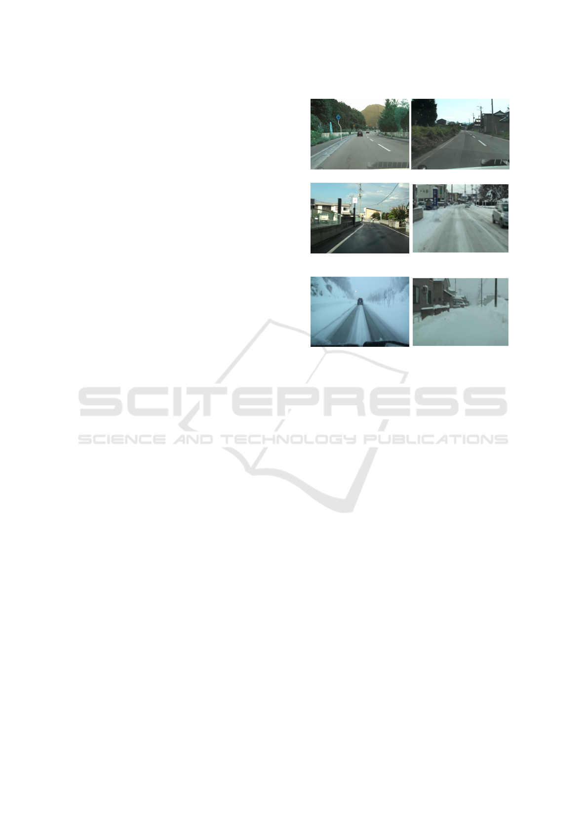
with snow. In these cases, it’s necessary to detect the

boundary line between the road and the roadside ob-

ject such as curbs (Fig. 1(a)), grasses (Fig. 1(b)),side

walls (Fig. 1(c)) and so on, instead of lane markers.

Especially, when the road is covered with snow, the

boundary with the snow side wall (Fig. 1(d)(e)(f))

needs to be detected since other roadside objects are

hidden by snow.

To detect a shoulder of the road, several methods

using color (M. A. Turk, D. G. Morgenthaler, K. D.

Gremban and M. Marra, 1988) and texture(J. Zhang

and H. Nagel, 1994) have been proposed. However,

when a road is covered with snow, it’s difﬁcult to

detect a road boundary by color and texture because

there are various kinds of snow surfaces, such as the

rough snow surface (Fig. 1(d)), the rutted snow sur-

face (Fig. 1(e)), and smooth white snow surface (Fig.

1(f)).

Since road shoulder is usually different in height

from a road plane, many methods using depth infor-

Goro, K. and Onoguchi, K.

Road Boundary Detection using In-vehicle Monocular Camera.

DOI: 10.5220/0006589703790387

In Proceedings of the 7th International Conference on Pattern Recognition Applications and Methods (ICPRAM 2018), pages 379-387

ISBN: 978-989-758-276-9

379

mation obtained by a stereo camera have been pro-

posed(D. Pfeiffer and U. Franke, 2010)(N. Einecke

and J. Eggert, 2013)(J. K. Suhr and H. G. Jung,

2013)(C. Guo, J. Meguro, Y. Kojima and T. Naito,

2013)(M. Enzweiler, P. Greiner, C. Knoppel and U.

Franke, 2013)(J. Siegemund, D. Pfeiffer, U. Franke

and W. Forstner, 2010). However, a stereo camera is

more expensive than a monocular camera and it takes

time and effort to install because strict calibration be-

tween two cameras is needed.

Road detection method based on semantic seg-

mentation has also been proposed. The literature (J.

M. Alvarez, T. Gevers and A. M. Lopez, 2010) pro-

poses the method which extracts road area by com-

bining 3D road cues, such as a horizon line, a vanish-

ing point and road geometry, and temporal road cues

in Bayesian framework. The literature (D. Hoiem,

A. A. Efros and M. Hebert, 2007) detects road area

by describing the 3D scene orientation of each im-

age region coarsely. The literatures (J. M. Alvarez,

Y. LeCum, T. Gevers and A. M. Lopez, 2012) and (J.

M. Alvarez, T. Gevers, Y. LeCum and A. M. Lopez,

2012) propose the method which detects road area by

Convolutional Neural Networks. The literature (D.

Levi, N. Garnett and E. Fetaya, 2015) proposed the

StixelNet whose input is Stixel instead of images. The

literature (C. Brust, S. Sickert, M. Simon, E. Rodner

and J. Denzler, 2015) detects road area by Convolu-

tional Patch Network whose input is a single image

patch extracted around a pixel to be labelled. In the

literatures (R. Mohan, 2014) and (G. L. Oliveira, W.

Burgard and T. Brox, 2016), road detection method

which combines deep deconvolutional and convolu-

tional neural networks is proposed. The literature (A.

Laddha, M. K. Kocamaz , L. E. N-serment, and M.

Hebert, 2016) proposes a boosting based method for

semantic segmentation of road scenes. The literature

(D. Costea and S. Nedevschi, 2017) proposes road de-

tection method which reduces human labeling effort

by a map-supervised approach. These methods show

considerably good results in various road scenes but

the results applied to the snow road are not shown.

This paper proposes the novel method that can de-

tect a road boundary from an image of a monocular

camera even if a road is covered with snow. Verti-

cal lines on an object whose height is different from

a road surface are projected onto slanting lines when

an input image is mapped to a road surface by the

inverse perspective transformation. Our method de-

tects a road boundary using this characteristic. We

introduce the degree of road boundary whose value

increases at the boundary with the area where slant-

ing edges are dense. Road boundary is extracted by

the Snakes using the degree of road boundary as im-

(a) Curbs (b) Grasses

snow surface)

(e) Snow side walls (Rutted

snow surface)

(f) Snow side walls

(Smooth snow surface)

Figure 1: Road boundary.

age forces.

This paper is organized as follows. Section 2

shows the outline of the proposed method. Section

3 explains how to create the Inverse Perspective Map-

ping (IPM) image from an input image. Section 4

explains the method to create IPM edge image that

emphasizes slant edges on road side objects. Section

5 explains the method to calculate the degree of road

boundary in each pixel of the IPM edge image. Sec-

tion 6 describes the method to track the road bound-

ary by the Snakes. Section 7 discusses experimental

results performed to several road scenes. Conclusions

are presented in Sect. 8.

2 THE OUTLINE OF THE

PROPOSED METHOD

Figure 2 shows the procedure of the proposed method.

The road boundary is detected in the Inverse Perspec-

tive Mapping (IPM) image. In the IPM image, the

patterns existing on the road surface are projected to

the shape viewed from the right overhead. On the

other hand, as shown in Fig. 3, road side objects or

obstacles whose height is different from the road sur-

face are projected to the shape falling backward from

the location where the obstacles touch the road plane.

Therefore, the proposed method detects the boundary

ICPRAM 2018 - 7th International Conference on Pattern Recognition Applications and Methods

380

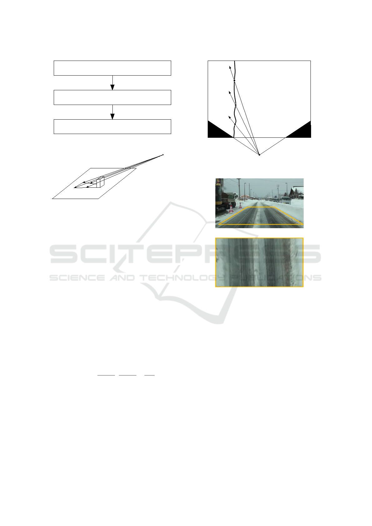
Figure 2: Outline of the proposed method.

Figure 3: Shape of projected area.

between dense areas of slant edges and sparse areas

of slant edges as the road boundary since a lot of slant

edges appear around a road side in the IPM image

(Fig. 4). First, the IPM edge image that emphasizes

slant edges on road side objects is created. Next, the

degree of road boundary whose value increases at the

boundary with the dense areas of slant edges is calcu-

lated in each pixel of the IPM edge image. Finally, the

road boundary is tracked by the Snakes whose image

force is the degree of road boundary.

3 CREATION OF IPM IMAGE

The inverse perspective mapping (IPM) image, which

overlooks a road surface, is created by inverse per-

spective transform. A point (x, y) in the image co-

ordinate system and a point (u, v) in the IPM image

coordinate system satisfy

(u, v) = (RX

x −V

y −V

−

lim

), (1)

where (V

) is the position of a vanishing point

in the image coordinate system, RX and RY are com-

pression or expansion rates for direction x and y, and

lim

is the lower limit of y-coordinate value in the im-

age(T. Yasuda and K. Onoguchi, 2012). Figure 5(b)

shows the IPM image created from Fig. 5(a). Param-

eters (V

), RX, RY and ylim are calibrated when

the camera is installed in the vehicle. Unless the cam-

era position changes, these parameter are ﬁxed. In ex-

Figure 4: Projection of vertical edges.

(a) Input image

(b) IPM image

Figure 5: Inverse perspective mapping.

periments, the IPM image whose size is 640 × 480 is

created from an input image whose size is 640 × 480.

4 CREATION OF IPM EDGE

IMAGE

In the smooth snow surface, both a road side and a

road surface contain only weak texture in the IPM im-

age, as shown in Fig. 6(b). To emphasize slant edges

around a road side, the IPM edge image E

AND

(u, v) is

created by the below preprocessing.

1. The vertical edge image E

(x, y) (Fig. 6(c)) is cre-

ated by applying the Sobel operator to the input

image I(x, y) (Fig. 6(a)). (x, y) is the coordinate

value of an image.

2. E

(x, y) is converted to the IPM image E

ipm

(u, v)

(Fig. 6(d)). (u, v) is the coordinate value of the

Road Boundary Detection using In-vehicle Monocular Camera

381

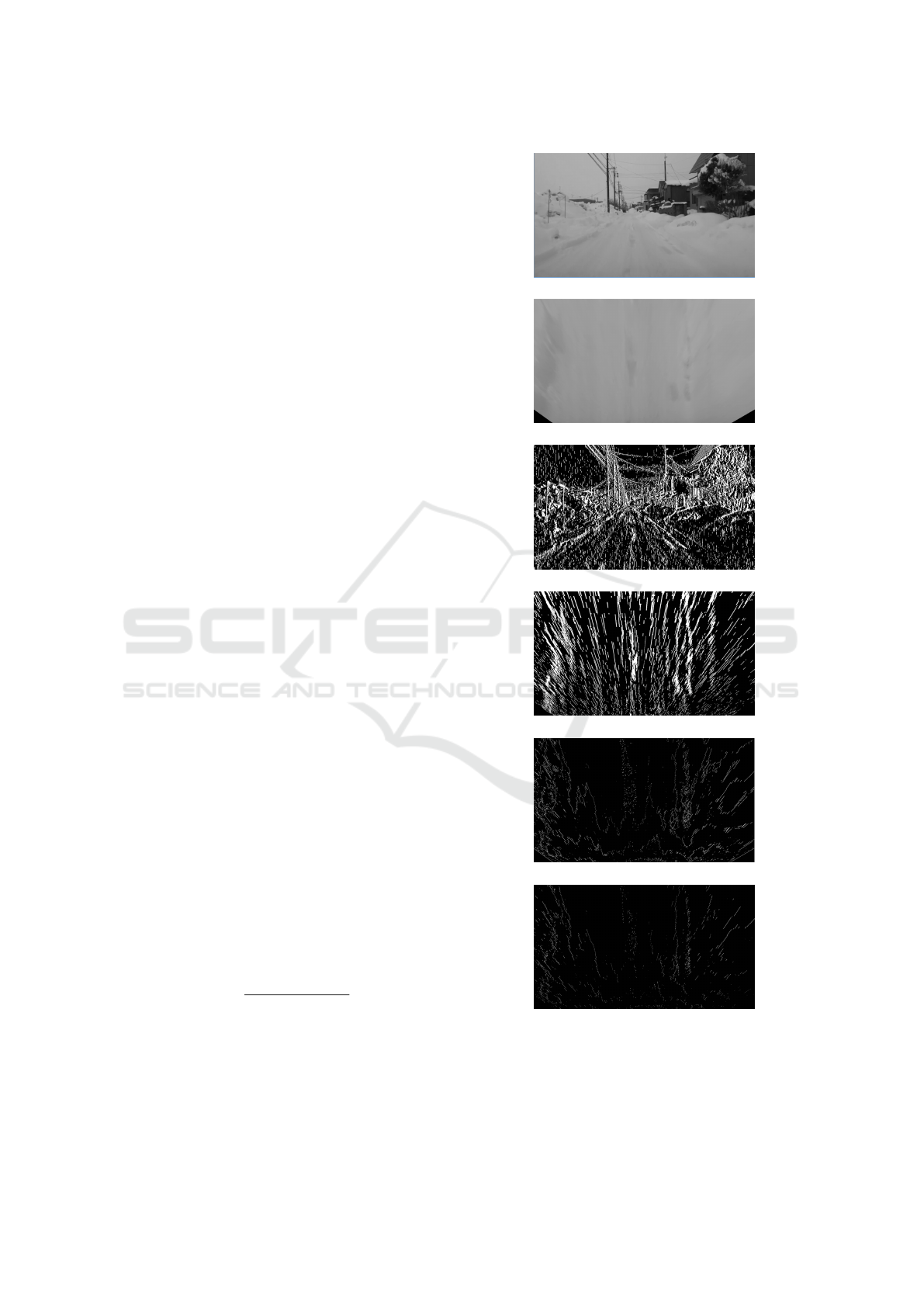
IPM image.

3. The slant edge image E

ipm

(u, v) (Fig. 6(e)) is cre-

ated by applying the Sobel operator to the IPM

image of I(x, y) (Fig. 6(b)).

4. The AND image E

AND

(u, v) of E

ipm

(u, v) and

ipm

(u, v) is created as the preprocessing im-

age for road boundary detection. Figure 6(f)

shows E

AND

(u, v) obtained from E

ipm

(u, v) and

ipm

(u, v).

Vertical edges on a roadside object are converted

into slant edges in the IPM image. On the other hand,

there are not many vertical edges on the road surface

converted into slant edges. Therefore, in E

AND

(u, v),

slant edges around a road side remains but slant edges

on a road surface are suppressed.

5 THE DEGREE OF ROAD

BOUNDARY

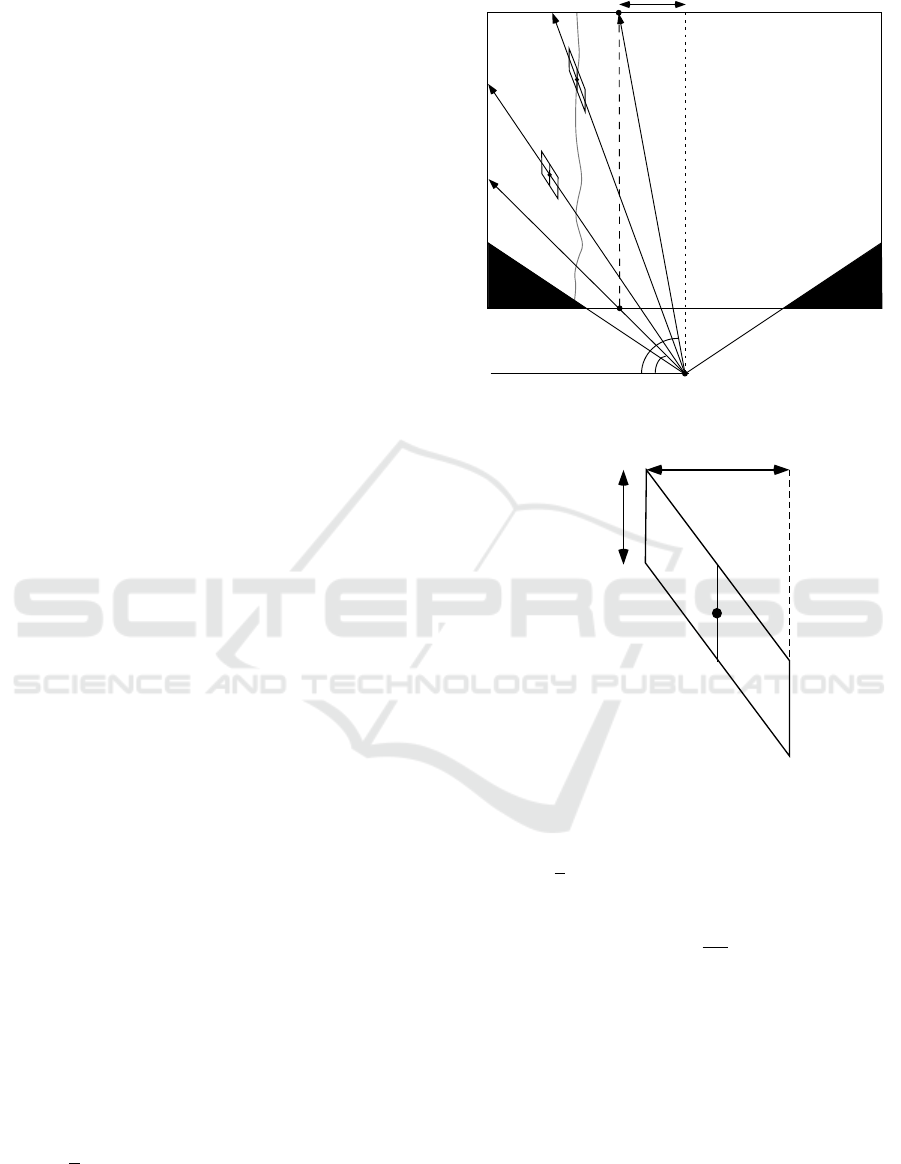
The vertical edge on the road side object is projected

as a shape falling backward radially around the cam-

era position, as shown in Fig.4. Therefore, in each

pixel of the IPM edge image, a parallelogram shaped

mask is set along a straight line L

connecting the

camera position C and each pixel P, as shown in Fig.7.

When parameters V

, V

, RX, RY and y

lim

for creating

the IPM image are ﬁxed, the straight line L

can be

determined in advance. An enlarged view of a par-

allelogram shaped mask is shown in Fig.8. Let the

length of the left and right sides of a mask be H, the

width between the left and right sides be W, the region

on the left side of the point P be R

and the region on

the right side of the point P be R

The road boundary is located on the left side of

the IPM image since vehicles drive on the left side of

the road in Japan. Since slant edges usually appear

densely on road side objects in the IPM edge image,

the number of edges in R

is large and the number

of edges in R

is small if the pixel P is around the

road boundary. For this reason, at each pixel P on the

left half of the IPM edge image, the degree of road

boundary BD is calculated by

BD =

+ (S

− N

)

+ S

, (2)

where N

is the number of edges in R

, N

is the

number of edges in R

, S

is the total number of pix-

els of R

and S

is the total number of pixels of R

The degree of road boundary BD increases around the

road boundary since it shows large value when N

large and N

is small.

(a) Smooth snow surface

(b) IPM image

(x, y)

(d) E

ipm

(u, v)

(e) E

ipm

(u, v)

(f) E

AND

(u, v)

Figure 6: Road boundary in smooth snow surface.

Since the camera position C is determined by

straight lines k

and k

indicating the bottom of

the IPM image as shown in Fig. 7, the slope θ of the

ICPRAM 2018 - 7th International Conference on Pattern Recognition Applications and Methods

382

straight line L

connecting the camera position C and

each pixel P can be calculated in advance. Therefore,

our method speeds up the calculation of N

and N

creating the table describing the information of paral-

lelogram shaped mask at each point P. At each pixel

P, the same W and H are used for the parallelogram

mask. The search angle around C is θ

< θ < θ

and

the degree θ is quantized in an integer value. Since

the parallelogram in the digital image is approximated

like a step as shown in Fig. 9, the shape of the paral-

lelogram mask generated by the parameter (W, H, θ)

is limited to several patterns T

(k = 0, . . . , n − 1). The

number of patterns n is uniquely determined when

W, H, θ

and θ

are ﬁxed.

At the pixel t

, v

)(i = 0, 1, . . . , w − 1) on the up-

per side of each pattern T

, a relative coordinate value

− u, v

− v) with the center P(u,v) of the mask is

calculated. Then, the table PT

(k, i)(0 ≤ k < n, 0 ≤

i < W − 1) in which u

− u is stored and the table

(k, i)(0 ≤ k < n, 0 ≤ i < W − 1) in which v

− v

is stored are created for parallelogram shaped mask.

At each pixel P(u, v) of the IPM edge image in

the range of θ

< θ < θ

, the slope θ of the straight

line L

is calculated in advance, and the index k of

the pattern T

corresponding to the angle θ is written

to two-dimensional array IA(u, v) whose size is same

as the IPM edge image. θ

and θ

are determined by

manually selecting the upper end A

max

and the lower

end A

min

of the shoulder in the IPM image which is

created from a vehicle parked on the shoulder (Fig.7).

In order to count the number of edges at high

speed, the line integral image S(u, v)(0 ≤ u <

IPM

, 0 ≤ v < H

IPM

) in the vertical direction is cre-

ated by applying the equation (3) to the IPM edge im-

age E

AND

(u, v)(0 ≤ u < W

IPM

, 0 ≤ v < H

IPM

S(u, v) =

∑

i=0

AND

(u, i) (3)

Using the line integral image S(u, v), the number of

edges E

num

on the vertical line between the red pixel

, v

) and the green pixel e

, u

+ H) in Fig. 9 is

calculated by the equation (4).

num

= S(u

, v

+ H) − S(u

, v

) (4)

Therefore, at each pixel P(u, v) of the IPM edge

image, N

and N

in the equation (2) are given by

equations 5 and 6 when IA(u, v) is equal to k.

−1

∑

i=0

(S(u + PT

(k, i), v + PT

(k, i) + H)

−S(u + PT

(k, i), v + PT

(k, i))) (5)

Figure 7: The degree of road boundary.

Figure 8: Parallelogram shaped mask.

W −1

∑

(S(u + PT

(k, i), v + PT

(k, i) + H)

−S(u + PT

(k, i), v + PT

(k, i))) (6)

Since both S

and S

are

W H

, the degree of road

boundary BD is calculated from equations (2), (5) and

(6). Figure 10(b) shows the example of the degree of

road boundary BD calculated from the IPM edge im-

age shown in Fig. 10(a). In this image, an BD is quan-

tized in the range from 0 and 255, and high intensity

shows high degree of road boundary.

6 ROAD BOUNDARY TRACKING

Our method detects and tracks the road boundary

by Snakes(M. Kass, A. Witkin and D. Terzopoulos,

Road Boundary Detection using In-vehicle Monocular Camera

383

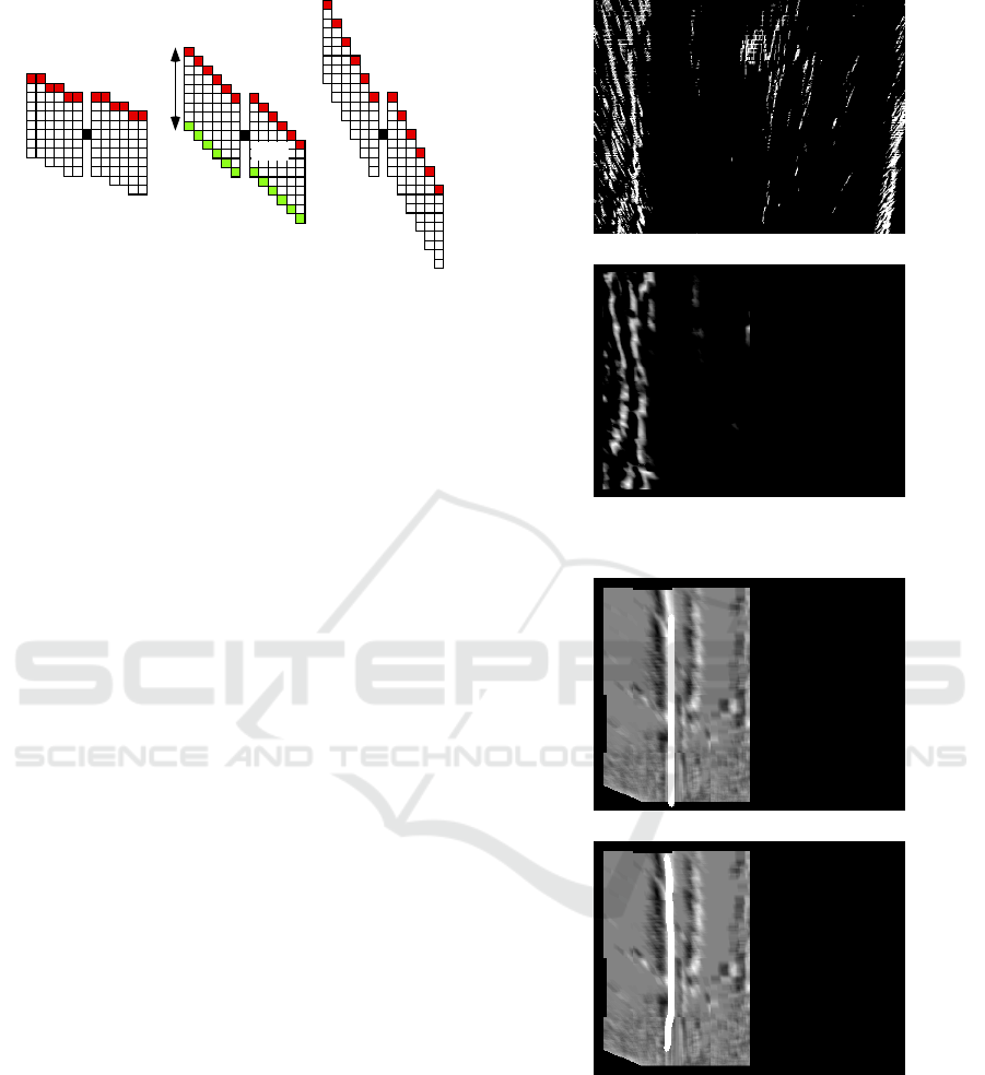
Figure 9: Parallelogram shaped mask in digital image.

1988) whose image force is the degree of road bound-

ary BD. First, in the BD image such as Fig. 10(b),

the intensity is accumulated vertically and the vertical

line passing through the peak is used as the initial po-

sition of the Snakes as shown in Fig. 11(a). The num-

ber of control points is 61 and the number of updates

is 10 per frame. Figure 11(b) shows the convergence

result of the Snakes.

7 EXPERIMENTS

We conducted experiments to detect the road bound-

ary from images taken by an in-vehicle monocular

camera. The KITTI dataset(KITTI, ) and our own

dataset including snow road scenes were used for

qualitative and quantitative evaluation.

7.1 Qualitative Evaluation

Figure 12 show some experimental results using the

KITTI dataset. Since Japanese roads are on the right

side, we detected the road boundary in the mirror im-

age. In each ﬁgure, the left is the detection result over-

laid on the input image with a magenta line and the

right is the ground truth of the road surface shown in

KITTI dataset. In Fig. 12(a), the curb is detected as

the road boundary correctly. In Fig. 12(c), the bound-

ary between the road surface and the roadside grass is

detected correctly. In Fig. 12(e), The boundary with

the parked vehicle is correctly detected.

Since snow road scene is not included in the

KITTI dataset, we built the dataset containing vari-

ous roads covered with snow. We call this dataset

HRB(Hirosaki Road Boundary) dataset. Figure 13

shows some experimental results using HRBD. In

each ﬁgure, the left is the detection result and the

right is the ground truth set manually in the IPM im-

age. The HRB dataset also contains road boundaries

such as the curb, the roadside grass and so on other

than snowy road. In Fig. 13(a) and (c), the curb

(a) IPM edge image

(b) The degree of road boundary

Figure 10: Example of the degree of road boundary.

(a) Initial position of Snakes

(b) Convergence result

Figure 11: Tracking result of road boundary.

and the roadside grass are detected correctly. Figure

13(e) shows the result in a sherbet-like snow surface,

Fig. 13(g) shows the result in a smooth snow surface

and Fig. 13(i) shows the result in the scene where

the road surface is not covered with snow but a lane

marker is occluded by the snow side wall. Although

lane markers are invisible in these scenes, the bound-

ary between the snow side wall and a road surface is

ICPRAM 2018 - 7th International Conference on Pattern Recognition Applications and Methods

384

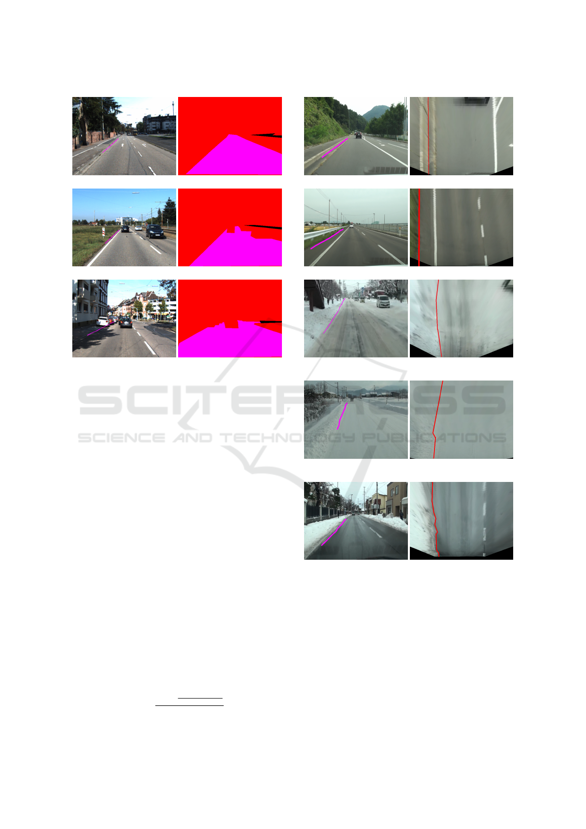
(a) Curb (b) Curb(Ground Truth)

(e) Parked vehicle (f) Parked vehicle(Ground

Truth)

Figure 12: Results of road boundary detection (KITTI

dataset).

detected correctly as a boundary of the driving lane.

7.2 Quantitative Evaluation

We evaluated the performance of the proposed

method quantitatively in the KITTI dataset and the

HRB dataset.

In the KITTI dataset, images containing road side

objects such as curbs, grasses, vehicles and so on were

used for evaluation. 127 frames of the curb and 56

frames of the other road side object including parked

vehicles were evaluated. Only the left side of the driv-

ing lane in the mirror image was compared with the

ground truth tracing the left boundary of the true road

area shown in the KITTI dataset.

The HRB dataset contains 100 frames of the curb,

161 frames of the road side grass and 142 frames of

the snow side wall. The ground truth was obtained by

tracing the road boundary manually in the IPM image.

The detection accuracy DA given by the equation

(7) is estimated in the IPM image. Therefore, the

ground truth for the KITTI dataset is projected onto

the IPM image.

DA =

∑

n−1

i=0

(i)−pt

(i)|

LaneWidth

(7)

(a) Curb (b) Curb(Ground Truth)

(e) Sherbet-like snow surface (f) sherbet-like snow sur-

face(Ground Truth)

(g) Smooth snow surface (h) Smooth snow sur-

face(Ground Truth)

(i) Wet surface (j) Wet surface(Ground

Truth)

Figure 13: Results of road boundary detection (HRB

dataset).

Where p

(i) is the u coordinate value of the control

point calculated by the snakes, pt

(i) is the u coor-

dinate value of the ground truth whose v coordinate

value is same as p

(i), n is the number of the control

points in the Snakes and LaneWidth is the width of

the driving lane in the IPM image.

Table 1 shows the detection accuracy DA in the

KITTI dataset. The average DA of all scenes is 0.088.

Road Boundary Detection using In-vehicle Monocular Camera

385

Table 1: Detection accuracy (KITTI dataset.)

# of frames DA

Curb 127 0.095

Other 56 0.071

Total 183 0.088

Table 2: Detection accuracy (HRB dataset.)

# of frames DA

Curb 100 0.046

Grass 161 0.118

Snow side wall 142 0.080

Total 403 0.087

This result shows that the error of 0.27m occurs when

the width of the driving lane is about 3m. However,

this result shows that a vehicle has some space to run

in the driving lane if the vehicle width is less than

2.5m. Therefore, the proposed method can also be

applied to ordinary vehicles.

Table 2 shows the detection accuracy DA in the

HRB dataset. The average DA of all scenes is 0.087

and DA of the snow side wall is 0.08. This result

shows that the proposed method is effective for road

boundary detection on snowy roads.

8 CONCLUSION

This paper proposed the method to detect the shoulder

line of a road including the boundary with the snow

side wall from an image of an in-vehicle monocular

camera. Vertical lines on an object whose height is

different from a road surface are projected onto slant-

ing lines when an input image is mapped to a road

surface by the inverse perspective mapping. The pro-

posed method detects a road boundary using this char-

acteristic. In the IPM edge image, the degree of road

boundary that responds strongly at the boundary with

the area where slant edges are dense is calculated

by using the parallelogram shaped mask. The road

boundary is tracked by the Snakes whose image force

is the degree of road boundary. Experimental results

using the KITTI dataset and our own dataset including

snow scenes show the effectiveness of the proposed

method. The future work is to improve the detection

accuracy of distant shoulder.

REFERENCES

A. Laddha, M. K. Kocamaz , L. E. N-serment, and M.

Hebert (2016). Map-supervised road detection. In

Proceedings of IV2016.

B. Hillel, R. Lerner, D. Levi, and G. Raz (2014). Recent

progress in road and lane detection: A survey. Ma-

chine Vision and Applications, 25(3):727–745.

C. Brust, S. Sickert, M. Simon, E. Rodner and J. Denzler

(2015). Convolutional patch networks with spatial

prior for road detection and urban scene understans-

ing. In Proceedings of VISAPP2015.

C. Guo, J. Meguro, Y. Kojima and T. Naito (2013). Cadas: a

multimodal advanced driver assistance system for nor-

mal urban streets based on road context understand-

ing. In Proceedings of IV2013, pages 228–235.

C. Kreucher and S. Lakshmanan (1999). Lana: A lane

extraction algorithm that uses frequency domain fea-

tures. IEEE Trans. on Robotics and Automation,

15(2):343–350.

D. Costea and S. Nedevschi (2017). Trafﬁc scene segmen-

tation based on boosting over multimodal low, inter-

mediate and high order multi-range channel features.

In Proceedings of IV2017.

D. Hoiem, A. A. Efros and M. Hebert (2007). Recovering

surface layout from an image. International Journal

of Computer Vision, 75(1):151–172.

D. Levi, N. Garnett and E. Fetaya (2015). Stixelnet: A depp

convolutional network for obstacle detection and road

segmentation. In Proceedings of BMVC2015.

D. Pfeiffer and U. Franke (2010). Efﬁcient representation

of trafﬁc scenes by means of dynamic stixels. In Pro-

ceedings of IV2010, pages 217–224.

G. L. Oliveira, W. Burgard and T. Brox (2016). Efﬁcient

deep models for monocular road segmentation. In

Proceedings of IROS2016, pages 586–595.

G. Thomas, N. Jerome and S. Laurent (2010). Frequency

ﬁltering and connected components charaterization

for zebra-crossing and hatched markings detection.

In Proceedings of ISPRS Commision III Symposium,

pages 43–47.

J. C. McCall and M. M. Trivedi (2006). Video-based lane

estimation and tracking for driver assistance: Survey,

system, and evaluation. IEEE Trans. on Intelligent

Transportation Systems, 7(1):20–37.

J. K. Suhr and H. G. Jung (2013). Noise resilient road sur-

face and free space estimation using dense stereo. In

Proceedings of IV2013, pages 461–466.

J. M. Alvarez, T. Gevers and A. M. Lopez (2010). 3d

scene priors for road detection. In Proceedings of

CVPR2010.

J. M. Alvarez, T. Gevers, Y. LeCum and A. M. Lopez

(2012). Road scene segmentation from a single im-

age. In Proceedings of ECCV2012, pages 376–389.

J. M. Alvarez, Y. LeCum, T. Gevers and A. M. Lopez

(2012). Semantic road segmentation via multi-scale

ensembles of learned features. In Proceedings of

ECCV2012, pages 586–595.

J. Siegemund, D. Pfeiffer, U. Franke and W. Forstner

(2010). Curb reconstruction using conditional random

ﬁelds. In Proceedings of IV2010, pages 203–210.

J. Zhang and H. Nagel (1994). Texture-based segmentation

of road images. In Proceedings of IV1994.

J.Douret, R. Labayrade, J. Laneurit and R. Chapuis (2005).

A reliable and robust lane detection system based on

ICPRAM 2018 - 7th International Conference on Pattern Recognition Applications and Methods

386

the parallel use of three algorithms for driving safety

assistance. In Proceedings of IAPR Conference on

Machine Vision Applications, pages 398–401.

KITTI. The KITTI Vision Benchmark Suite.

http://www.cvlibs.net/datasets/kitti/index.php.

M. A. Turk, D. G. Morgenthaler, K. D. Gremban and M.

Marra (1988). Vita-a vision system for autonomous

land vehicle navigation. IEEE Trans. on Pattern Anal-

ysis and Machine Intelligence, 10(3).

M. Bertozzi, A. Broggi, M. Cellario, A. Fascioli, P. Lom-

bardi and M. Porta (2002). Artiﬁcial vision in road

vehicles. Proceedings of the IEEE, 90(7):1258–1271.

M. Bertozzi and A. Broggi (1998). Gold: A parallel real-

time stereo vision system for generic obstacle and lane

detection. IEEE Trans. on Image Processing, 7(1):62–

81.

M. Enzweiler, P. Greiner, C. Knoppel and U. Franke (2013).

Towards multi- cue urban curb recognition. In Pro-

ceedings of IV2013, pages 902–907.

M. Kass, A. Witkin and D. Terzopoulos (1988). Snakes:

Active contour models. International Journal of Com-

puter Vision, 1(4):321–331.

M. Meuter, S. Muller-Schneiders, A. Mika, S. Hold, C.

Numm and A. Kummert (2009). A novel approach

to lane detection and tracking. In Proceedings of

ITSC2009, pages 582–587.

N. Einecke and J. Eggert (2013). Stereo image warping

for improved depth estimation of road surfaces. In

Proceedings of IV2013, pages 189–194.

R. Mohan (2014). Deep deconvolutional networks for scene

parsing. In ArXiv.org.

S. Hold, S. Gormer, A. Kummert, M. Meuter, S. Muller-

Schneiders (2010). Ela - an exit lane assistant for

adaptive cruise control and navigation systems. In

Proceedings of ITSC2010, pages 629–634.

T. Yasuda and K. Onoguchi (2012). Lane estimation based

on lane marking recognition. In Proceedings of ITS

World Congress 2012.

Z. W. Kim (2008). Robust lane detection and tracking

in challenging scenarios. IEEE Trans. on Intelligent

Transportation Systems, 9(1):16–26.

Road Boundary Detection using In-vehicle Monocular Camera

387