Deep Learning Policy Quantization

Jos van de Wolfshaar, Marco Wiering and Lambert Schomaker

∗

Institute of Artiﬁcial Intelligence and Cognitive Engineering, University of Groningen, The Netherlands

Keywords:

Reinforcement Learning, Deep Learning, Learning Vector Quantization, Nearest Prototype Classiﬁcation,

Deep Reinforcement Learning, Actor-Critic.

Abstract:

We introduce a novel type of actor-critic approach for deep reinforcement learning which is based on learning

vector quantization. We replace the softmax operator of the policy with a more general and more ﬂexible

operator that is similar to the robust soft learning vector quantization algorithm. We compare our approach

to the default A3C architecture on three Atari 2600 games and a simplistic game called Catch. We show that

the proposed algorithm outperforms the softmax architecture on Catch. On the Atari games, we observe a

nonunanimous pattern in terms of the best performing model.

1 INTRODUCTION

Deep reinforcement learning (DRL) is the marriage

between deep learning (DL) and reinforcement learn-

ing (RL). Combining the two enables us to create self-

learning agents that can cope with complex environ-

ments while using little or no feature engineering. In

DRL systems, the salient features in the data are ex-

tracted implicitly by a deep neural network (DNN).

After the ﬁrst major successes in DRL with deep Q-

learning (Mnih et al., 2013; Mnih et al., 2015), many

alternative approaches have been explored which are

well summarized in (Li, 2017).

On a coarse-grained level, decision making as

done by RL agents can be related to classiﬁcation.

One particular class of classiﬁcation algorithms is

known as nearest prototype classiﬁcation (NPC). The

most prominent NPC algorithm is learning vector

quantization (LVQ) (Kohonen, 1990; Kohonen, 1995;

Kohonen et al., 1996). As opposed to linearly sepa-

rating different kinds of inputs in the ﬁnal layer of a

neural network, LVQ chooses to place possibly mul-

tiple prototype vectors in the input space X . Roughly

speaking, a new input~x is then classiﬁed by looking at

the nearest prototypes in X . This particular classiﬁca-

tion scheme could in principle be used for reinforce-

ment learning with some modiﬁcations. More specif-

ically, we will look at how it can be used to frame

the agent’s decision making as an LVQ problem. In

∗

This project has received funding from the European

Union’s Horizon 2020 research and innovation programme

under grant agreement No 662189 (Mantis).

that case, the prototypes will be placed in a feature

space H ⊆ R

in which we compare the prototypes to

nearby hidden activations

h of a DNN.

Recently, the asynchronous advantage actor-critic

(A3C) algorithm was introduced. The actor-critic al-

gorithm uses a softmax operator to construct its pol-

icy approximation. In this paper, we explore an alter-

native policy approximation method which is based

on LVQ (Kohonen, 1990; Kohonen, 1995; Kohonen

et al., 1996). We accomplish this by replacing the

softmax operator with a learning policy quantization

(LPQ) layer. In principle, the proposed method al-

lows for a more sophisticated separation of the fea-

ture space. This, in turn, could yield a superior policy

when compared to the separation that a softmax oper-

ator can accomplish.

We explore several variations to the LPQ layer

and evaluate them on two different kinds of domains.

The ﬁrst domain is a self-implemented version of the

Catch game (Mnih et al., 2014). The second domain

consists of three Atari 2600 games. We show that the

LPQ layer can yield better results on Catch, whereas

the results on Atari 2600 are not unanimously in favor

of any of the approaches.

We now provide an outline of this paper. First, we

discuss relevant literature in Section 2. We then cover

basic reinforcement learning deﬁnitions in Section 3.

Then, we describe the workings of LPQ in Section 4.

Our experiments are covered in Section 5. Finally, we

reﬂect on the outcomes and we provide suggestions

for future work on LPQ in Section 6.

122

Wolfshaar, J., Wiering, M. and Schomaker, L.

Deep Learning Policy Quantization.

DOI: 10.5220/0006592901220130

In Proceedings of the 10th International Conference on Agents and Artiﬁcial Intelligence (ICAART 2018) - Volume 2, pages 122-130

ISBN: 978-989-758-275-2

2 RELATED WORK

This section covers related work in the ﬁeld of deep

reinforcement learning. More speciﬁcally, we discuss

the asynchronous advantage A3C algorithm and LVQ.

2.1 Asynchronous Advantage

Actor-critic

Despite the signiﬁcant successes that have been ob-

tained through the usage of a DQN with different

kinds of extensions, the replay memory itself has

some disadvantages. First of all, a replay memory

requires a large amount of computer memory. Sec-

ond, the amount of computation per real interaction

is higher and third, it restricts the applicable algo-

rithms to be off-policy RL methods. In (Mnih et al.,

2016), the authors introduce asynchronous algorithms

for DRL. By running multiple agents in their own in-

stance of the environment in parallel, one can decor-

relate subsequent gradient updates, which fosters the

stability of learning. This opens the way for on-policy

methods such as Sarsa, n-step methods and actor-

critic methods. Their best performing algorithm is

the asynchronous advantage actor-critic method with

n-step returns.

A major disadvantage of single step methods such

as DQN is that in the case of a reward, only the value

of the current state-action pair (s,a) is affected di-

rectly, whereas n-step methods directly incorporate

multiple state-action pairs into a learning update. In

(Mnih et al., 2016), it is shown that the A3C algorithm

outperforms many preceding alternatives. Moreover,

they explore the A3C model in other domains such

as a Labyrinth environment which is made publicly

available by (Beattie et al., 2016), the TORCS 3D car

racing simulator (Wymann et al., 2000) and MuJoCo

(Todorov et al., 2012) which is a physics simulator

with continuous control tasks. The wide applicabil-

ity of their approach supports the notion that A3C is a

robust DRL method.

In (Jaderberg et al., 2016), it is shown that the per-

formance of A3C can be substantially improved by in-

troducing a set of auxiliary RL tasks. For these tasks,

the authors deﬁned pseudo-rewards that are given for

feature control tasks and pixel control tasks. The in-

clusion of these auxiliary tasks yields an agent that

learns faster. The authors show that reward predic-

tion contributes most to the improvement over A3C,

whereas pixel control had the least effect of improve-

ment.

2.2 Learning Vector Quantization

LVQ algorithms were designed for supervised learn-

ing. They are mainly used for classiﬁcation tasks.

This section will brieﬂy discuss LVQ and the most

relevant features that inspired us to develop LPQ.

2.3 Basic LVQ

We assume we have some feature space H ⊆ R

Let

h be a feature vector of a sample in H . Now

given a set of prototypes {~w

,~w

,. ..,~w

} and cor-

responding class assignments given by the function

c : H 7→{0,1,... ,#classes−1}, we update prototypes

as follows:

←~w

+ η(t)(

h −~w

), (1)

←~w

−η(t)(

h −~w

), (2)

where ~w

is the closest prototype of the same class

h (so c(~w

) = c(

h)), and ~w

is the closest proto-

type of another class (so c(~w

) 6= c(

h)). Similar to the

notation in (Kohonen, 1990), we use a learning rate

schedule η(t). In LVQ 2.1, these updates are only

performed if the window condition is met, which is

that min{d

} > `, where ` is some prede-

ﬁned constant. Here d

= d(~w

h) is the distance of

the current vector

h to the prototype ~w

. The same dis-

tance function is used to determine which prototypes

are closest.

Unseen samples are classiﬁed by taking the class

label of the nearest prototype(s). Depending on the

speciﬁc implementation, a single or multiple nearby

prototypes might be involved. Note that the set of pro-

totypes might be larger than the number of classes.

This is different from a softmax operator, where the

number of weight vectors (or prototypes) must corre-

spond to the number of classes.

2.4 Generalized Learning Vector

Quantization

One of the major difﬁculties with the LVQ 2.1 al-

gorithm is that the prototypes can diverge, which

eventually renders them completely useless for the

classiﬁer. Generalized learning vector quantization

(GLVQ) was designed to overcome this problem

(Sato and Yamada, 1996). Sato and Yamaha deﬁne

the following objective function to be minimized:

∑

Φ(µ

) with µ

(i)

−d

(i)

−

(i)

+ d

(i)

−

, (3)

Deep Learning Policy Quantization

123

where Φ : R 7→ R is any monotonically increasing

function, d

(i)

= min

:c(~w

)=c(

h,~w

) is the dis-

tance to the closest correct prototype and d

(i)

−

min

:c(~w

)6=c(

h,~w

) is the distance to the closest

prototype with a wrong label. In (Sato and Yamada,

1996) it is shown that for certain choices for the dis-

tance function, the algorithm is guaranteed to con-

verge.

2.5 Deep Learning Vector Quantization

Recently, (De Vries et al., 2016) proposed a deep

LVQ approach in which the distance function is de-

ﬁned as follows:

h,~w) = kf (x;

) −~wk

, (4)

where f is a DNN with parameter vector

and

h =

f (~x;

). Their deep LVQ method serves as an alter-

native to the softmax function. The softmax function

has a tendency to severely extrapolate such that cer-

tain regions in the parameter space attain high conﬁ-

dences for certain classes while there is no actual data

that would support this level of conﬁdence. Moreover,

they propose to use the objective function as found

in generalized LVQ. They show that a DNN with a

GLVQ cost function outperforms a DNN with a soft-

max cost function. In particular, they show that their

approach is signiﬁcantly less sensitive to adversarial

examples.

An important design decision is to no longer de-

ﬁne prototypes in the input space but in the feature

space. This saves forward computations for proto-

types and can simplify the learning process as the fea-

ture space is generally a lower-dimensional represen-

tation compared to the input itself.

2.6 Robust Soft Learning Vector

Quantization

Rather than having an all-or-nothing classiﬁcation,

class conﬁdences can also be modelled by framing

the set of prototypes as deﬁning a density function

over the input space X . This is the idea behind robust

soft learning vector quantization (RSLVQ) (Seo and

Obermayer, 2003).

3 REINFORCEMENT LEARNING

BACKGROUND

In this paper we consider reinforcement learning

problems in which an agent must behave optimally in

a certain environment (Sutton and Barto, 1998). The

environment deﬁnes a reward function R : S 7→R that

maps states to scalar rewards. The state space consists

of all possible scenarios in the Atari games. This im-

plies that we are dealing with a discrete state space. In

each state, the agent can pick an action a from a dis-

crete set A. We say that an optimal agent maximizes

its expected cumulative reward. The cumulative re-

ward of a single episode is also known as the return

∑

∞

k=0

t+k

, where R

is the reward obtained at

time t. An episode is deﬁned by a sequence of states,

actions and rewards. An episode ends whenever a ter-

minal state is reached. For Atari games, a typical ter-

minal state is when the agent is out of lives or when

the agent has completed the game. An agent’s policy

π : S ×A 7→ [0,1] assigns probabilities to all state-

action pairs.

The state-value function V

(s) gives the expected

reward for being in state s and following policy π

afterwards. The optimal value function V

∗

(s) maxi-

mizes this expectation. The state-action value func-

tion Q

(s,a) gives the expected reward for being in

state s, taking action a and following π afterwards.

The optimal state-action value function maximizes

this expectation. The optimal policy maximizes the

state-value function at all states.

For reinforcement learning with video games, the

number of different states can grow very large due to

the high dimensionality of the environment. There-

fore, we require function approximators that allow us

to generalize knowledge from similar states to unseen

situations. The function approximators can be used

to approximate the optimal value functions or to ap-

proximate the optimal policy directly. In deep rein-

forcement learning, these function approximators are

DNNs, which are typically more difﬁcult to train ro-

bustly than linear function approximators (Tsitsiklis

et al., 1997).

The A3C algorithm is a policy-based model-free

algorithm. This implies that the agent learns to be-

have optimally through actual experience. Moreover,

the network directly parameterizes the policy, so that

we do not require an additional mechanism like ε-

greedy exploration to extract a policy. Like any other

actor-critic method, A3C consists of an actor that ap-

proximates the policy with π(s,a;

) and a critic that

approximates the value with V (s;

). In the case of

A3C, both are approximated with a single DNN. In

other words, the hidden layers of the DNN are shared

between the actor and the critic. We provide a detailed

description of the A3C architecture in Section 5.2.

ICAART 2018 - 10th International Conference on Agents and Artiﬁcial Intelligence

124

4 LEARNING POLICY

QUANTIZATION

This section introduces a new kind of actor-critic al-

gorithm: learning policy quantization (LPQ). It draws

inspiration from LVQ (Kohonen, 1990; Kohonen,

1995; Kohonen et al., 1996). LVQ is a supervised

classiﬁcation method in which some feature space H

is populated by a set of prototypes W = {~w

}

i=1

Each prototype belongs to a particular class so that

c(~w

) gives the class belonging to ~w

To a certain extent, the parameterized policy of a

DNN in A3C, denoted π(s,a;

), draws some paral-

lels with a DNN classiﬁer. In both cases, there is a

certain notion of conﬁdence toward a particular class

label (or action) and both are often parameterized by

a softmax function. Moreover, both can be optimized

through gradient descent. We will now generalize the

actor’s output to be compatible with an LVQ classiﬁ-

cation scheme. Let us ﬁrst rephrase the softmax func-

tion as found in the standard A3C architecture:

π(s,a;

) =

exp



L−1

+ b



∑

exp



L−1

+ b



, (5)

where h

L−1

is the activation of the last hidden layer,

is a bias for action a and ~w

is the weight vector for

action a. Now consider the more general deﬁnition:

π(s,a;

) =

∑

i:c(~w

)=a

exp



ς(~w

L−1

)



∑

exp



ς(~w

L−1

)



, (6)

where ς is a similarity function. Now, we allow mul-

tiple prototypes to belong to the same action by sum-

ming the corresponding exponentialized similarities.

In this form, the separation of classes in the feature

space can be much more sophisticated than a normal

softmax operator. We have chosen to apply such ex-

ponential normalization similar to a softmax function

which makes the output similar to RSLVQ (Seo and

Obermayer, 2003). This provides a clear probabilistic

interpretation that has proven to work well for super-

vised learning.

We also assess the LPQ equivalent of generalized

LVQ. The generalized learning policy quantization

(GLPQ) output is computed as follows:

π(s,a;

) =

∑

i:c(~w

)=a

exp



−ς

⊥

+ς

⊥



∑

exp



−ς

⊥

+ς

⊥



(7)

∑

i:c(~w

)=a

exp(τµ

)

∑

(τµ

)

, (8)

where we have abbreviated ς(~w

L−1

) with ς

and

where ς

⊥

= max

j6=i

. Using the closest proto-

types of another class (ς

⊥

) puts more emphasis on

class boundaries. During our initial experiments, we

quickly noticed that the temperature τ was affecting

the magnitude of the gradients signiﬁcantly, which

could lead to poor performance for values far from

τ = 1. We compensated for this effect by multiplying

the policy loss used in gradient descent with a factor

1/τ. We will explain the importance of this τ param-

eter in Section 4.2.

4.1 Attracting or Repelling without

Supervision

Note that there is a subtle yet important difference in

the deﬁnition of Equation (7) compared to the deﬁni-

tion in Equation (3). We can no longer directly deter-

mine whether a certain prototype ~w

is correct as we

do not have supervised class labels anymore.

The obvious question that comes to mind is: how

should we determine when to move a prototype to-

ward some hidden activation vector

h? The answer

is provided by the environment interaction and the

critic. To see this, note that the policy gradient the-

orem (Sutton et al., 2000) already justiﬁes the follow-

ing:

∆

← ∆

−∇

logπ(a

;

)(G

(n)

−V (s

;

)),

(9)

where G

(n)

∑

n−1

k=0

t+k

+ γ

V (s

t+n

;

) is the n-

step return obtained through environment interaction

and V (s

;

) is the output of the critic. This expres-

sion accumulates the negative gradients of the actor’s

parameter vector

. When these negative gradients

are plugged into a gradient descent optimizer such as

RMSprop (Tieleman and Hinton, 2012), the result-

ing behavior is equivalent to gradient ascent, which

is required for policy gradient methods. It is impor-

tant to realize that all prototypes ~w

are included in

the parameter vector

. The factor (G

(n)

−V(s

;

))

is also known as the advantage. The advantage of a

certain action a gives us the relative gain in expected

return after taking action a compared to the expected

return of state s

. In other words, a positive advantage

corresponds to a correct prototype, whereas a nega-

tive advantage would correspond to a wrong proto-

type. Intuitively, applying Equation (9) now corre-

sponds to increasing the result of µ

(that is by attract-

ing ~w

and repelling ~w

⊥

) whenever the advantage is

positive and decreasing the result of µ

(that is by re-

pelling ~w

and attracting ~w

⊥

) whenever the advantage

is negative.

Hence, the learning process closely resembles that

of GLVQ while we only modify the construction of

π(s,a;

). Note that a similar argument can be made

Deep Learning Policy Quantization

125

for LPQ with respect to RSLVQ (Seo and Obermayer,

2003).

4.2 Temperature for GLPQ

An interesting property of the relative distance mea-

sure as given by µ

, is that it is guaranteed to be in the

range [−1,1]. Therefore, we can can show that the

maximum value of the actor’s output is:

maxπ(s, a;

) =

exp(2τ)

exp(2τ)+ |A|−1

, (10)

where we have assumed that each action has exactly k

prototypes. Alternatively, one could determine what

the temperature τ should be given some desired max-

imum p:

τ =



−

p(|A|−1)

p −1



. (11)

Hence, we can control the rate of stochasticity

through the parameter τ in a way that is relatively sim-

ple to interpret when looking at the value of p. For

further explanation regarding Equations (10) and (11)

see the Appendix. We will use Equation (11) to deter-

mine the exact value of τ. In other words, τ is not part

of our hyperparameters, whereas p is part of it.

5 EXPERIMENTS

This section discusses the experiments that were per-

formed to assess different conﬁgurations of LPQ. We

ﬁrst describe our experiment setup in terms of envi-

ronments, models and hyperparameters. Finally, we

present and discuss our results.

5.1 Environments

We have two types of domains. The ﬁrst domain,

Catch, is very simplistic and was mainly intended to

ﬁnd proper hyperparameter settings for LPQ, whereas

the second domain, Atari, is more challenging.

5.1.1 Catch

For testing and hyperparameter tuning purposes, we

have implemented the game Catch as described in

(Mnih et al., 2014). In our version of the game, the

agent only has to catch a ball that goes down from

top to bottom, potentially bouncing off walls. The

world is a 24 ×24 grid where the ball has a vertical

speed of v

= −1 cell/s and a horizontal speed of

∈ {−2,−1, 0,1,2}. If the agent catches the ball by

moving a little bar in between the ball and the bottom

Figure 1: Screenshot of the Catch game that is used in our

experiments.

of the world, the episode ends and the agent receives

a reward of +1. If the agent misses the ball, the agent

obtains a zero reward. With such a game, a typical

run of the A3C algorithm only requires about 15 min-

utes of training time to reach a proper policy. For our

experiments, we resize the 24 ×24 world to have the

size of 84 ×84 pixels per frame. See Figure 1 for an

impression of the game.

5.1.2 The Arcade Learning Environment

To assess the performance of our proposed method

in more complex environments, we also consider a

subset of Atari games. The Arcade Learning Envi-

ronment (Bellemare et al., 2013) is a programmatic

interface to an Atari 2600 emulator. The agent re-

ceives a 210 ×160 RGB image as a single frame. The

observation is preprocessed by converting each frame

to a grayscale image of 84 ×84. Each grayscale im-

age is then concatenated with the 3 preceding frames,

which brings the input volume at 84 ×84 ×4. In be-

tween these frames, the agent’s action is repeated 4

times.

We have used the gym package (Brockman et al.,

2016) to perform our experiments in the Atari do-

main. The gym package provides a high-level Python

interface to the Arcade Learning Environment (Belle-

mare et al., 2013). For each game, we considered

the version denoted XDeterministic-v4, where X is the

name of the game. These game versions are available

since version 0.9.0 of the gym package and should

closely reﬂect the settings as used in most of the DRL

research on Atari since (Mnih et al., 2013). We have

run our experiments on Beam Rider, Breakout and

Pong.

5.2 Models

In our experiments, we compare three types of agents.

The ﬁrst agent corresponds to the A3C FF agent of

(Mnih et al., 2016), which has a feed-forward DNN.

It is the only agent that uses the regular softmax op-

erator, so we refer to it as A3C Softmax from hereon.

The other two agents are A3C LPQ and A3C GLPQ,

ICAART 2018 - 10th International Conference on Agents and Artiﬁcial Intelligence

126

which correspond to agents using the output operators

as deﬁned in Equation (6) and Equation (7) respec-

tively. Note that the A3C FF agent forms the basis

of our models, meaning that we use the exact same

architecture for the hidden layers as in (Mnih et al.,

2016). Only the output layers differ among the three

models. The ﬁrst convolutional layer has 32 kernels

of size 8 ×8 with strides 4 ×4, the second convolu-

tional layer has 64 kernels of size 4 ×4 with strides

2×2 and the ﬁnal layer is a fully connected layer with

256 units. All hidden layers use a ReLU nonlinearity

(Nair and Hinton, 2010).

Learning takes place by accumulating the gradi-

ents in minibatches of t

max

steps. The policy gradients

are accumulated through Equation (9) minus an en-

tropy factor ∇

βH(π(s

;

)) added to the right hand

side. The β parameter controls the relative impor-

tance of the entropy. The entropy factor encourages

the agent to explore (Williams and Peng, 1991).

The critic’s gradients are accumulated as follows:

∆

← ∆

+ ∇

(n)

−V (s

;

))

. (12)

After a minibatch of t

max

steps through Equation (9)

and (12), the accumulated gradients are used to update

the actual values of θ

and θ

. This is accomplished

by adding these terms together for any weights that

are shared in both the actor and the critic and adap-

tively rescaling the resulting gradient using the RM-

Sprop update:

~m ←α~m + (1 −α)∆

, (13)

θ ←

θ −η

∆θ/

√

~m + ε, (14)

where ~m is the vector that contains a running average

of the squared gradient and ε > 0 is a numerical stabil-

ity constant, α is the decay parameter for the running

average of the squared gradient and η is the learning

rate (Tieleman and Hinton, 2012). It is important to

realize that

theta contains the parameters of both the

actor and the critic. The squared gradients are initial-

ized at a zero vector and their values are shared among

all threads as proposed by (Mnih et al., 2016).

5.3 Hyperparameters

The reader might notice that a lot of parameters must

be preconﬁgured. We provide an overview in Table

1. Note that the weight initialization’s U refers to a

uniform distribution and ρ =

√

f an

. The f an

cor-

responds to the number of incoming connections for

each neuron. The temperature τ is determined through

using Equation (11). We linearly increase p

from

to p

max

. As is customary ever since the work by

(Mnih et al., 2013), we anneal the learning rate lin-

early between t = 0 and t = T

max

to zero.

Table 1: Overview of default settings for hyperparameters.

Name Symbol Value

Learning rate η 7 ·10

−4

Discount factor γ 0.99

RMSprop decay α 0.99

RMSprop stability ε 0.1

Entropy factor β 0.01

Steps lookahead t

max

Total steps ALE T

max

1 ·10

Total steps Catch T

max

1 ·10

Frames per observation NA 4

Action repeat ALE NA 4

Action repeat Catch NA 1

Number of threads NA 12

Prototypes per action NA 16

Similarity function ς(

h,~w) −

∑

−w

)

Max π GLPQ t = 0 p

0.95

Max π GLPQ t = T

max

0.99

Weight initialization NA U [−ρ, ρ]

Bias initialization NA 0

5.4 Results

For all our experiments, a training epoch corresponds

to 1 million steps for Atari and 50,000 for Catch.

Note that a step might result in multiple frames of

progress depending on the action repeat conﬁgura-

tion. At each training epoch, we evaluate the agent’s

performance by taking the average score of 50 envi-

ronment episodes.

5.4.1 Catch

First, we consider the Catch game as described in Sec-

tion 5.1.1. To get a better insight into the robustness

of each model, we consider a learning rate sweep in

which we vary the learning rate by sampling it from a

log-uniform distribution between 10

−6

and 10

−2

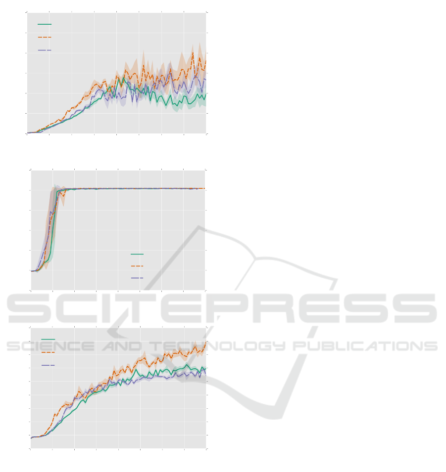
Similarity Functions. Figure 2 shows the aver-

age score for the learning rate sweep with different

similarity functions combined with the LPQ layer.

We looked at the Euclidean similarity ς(

h,~w) =

−

(

h −~w)

(

h −~w), the squared Euclidean similar-

ity ς(

h,~w) = −(

h −~w)

(

h −~w) and the Manhattan

similarity ς(

h,~w) = −

∑

−w

It is clear that the squared Euclidean similarity

works better than any other similarity function. More-

over, it attains good performance for a wide range of

learning rates. Hence, this is the default choice for

the remainder of our experiments. The second best

performing similarity measure is the Manhattan sim-

ilarity. This result corresponds with the theoretical

ﬁndings in (Sato and Yamada, 1996).

Deep Learning Policy Quantization

127

−6.0 −5.5 −5.0 −4.5 −4.0 −3.5 −3.0 −2.5 −2.0

log

(η)

0.0

0.2

0.4

0.6

0.8

1.0

Mean score ﬁnal 5 evaluations

Similarity functions

Euclidean

Manhattan

Squared Euclidean

Figure 2: Comparison between different similarity func-

tions for the LPQ model: performance score as a function

of the learning rate. The lines are smoothly connected be-

tween the evaluations of different runs. Note that for re-

porting each of these scores, we took the average evaluation

result of the ﬁnal 5 training epochs. A training epoch corre-

sponds to 50,000 steps.

Softmax, LPQ and GLPQ. Figure 3 displays the

learning rate sweep with a softmax architecture, an

LPQ architecture and a GLPQ architecture. We can

see that especially for lower learning rates between

−5

and 10

−4

, the GLPQ model seems to outper-

form the softmax and LPQ models. This could be

caused by the fact that the relative distance measure

puts more emphasis on class boundaries, which leads

to larger gradients for the most relevant prototypes.

The average across all learning rates between

−5

and 10

−2

is shown in Table 2, which also con-

ﬁrms that the GLPQ model outperforms the others.

GLPQ attains a score of 0.81 on average on the last 5

runs for any learning rate. This corresponds to catch-

ing the ball about 4 out of 5 times.

Table 2: Average ﬁnal evaluation scores across the full

learning rate sweep for LPQ, GLPQ and A3C with standard

deviations.

Model Score average (±σ)

Softmax 0.73 ±0.28

LPQ 0.72 ±0.28

GLPQ 0.81 ±0.21

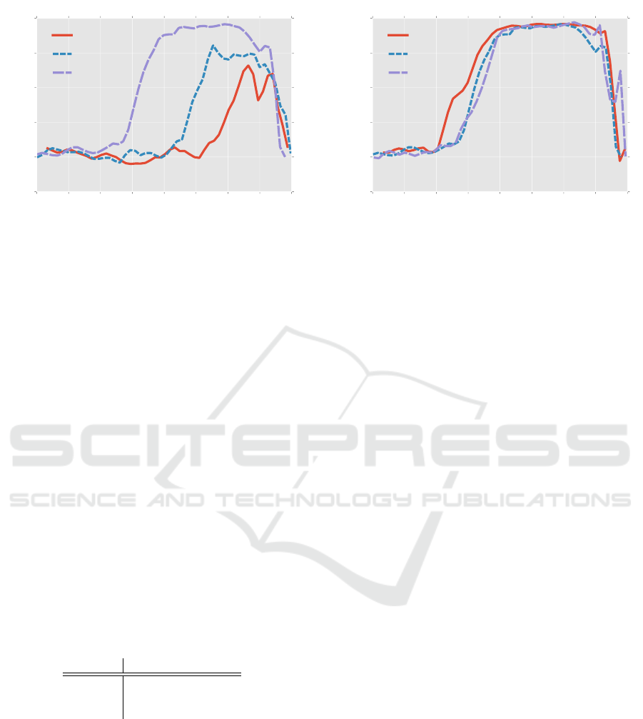
5.4.2 Atari

The results are shown in Figure 4. We have only

considered 3 games due to constraints in terms of

resources and time. It can be seen that GLPQ and

LPQ generally train slower than the default architec-

ture for Beam Rider and Breakout. For Breakout, the

ﬁnal performance for LPQ and A3C softmax is simi-

lar. For Beam Rider, GLPQ starts improving consid-

erably slower than LPQ and FF, but surpasses LPQ

−6.0 −5.5 −5.0 −4.5 −4.0 −3.5 −3.0 −2.5 −2.0

log

(η)

0.0

0.2

0.4

0.6

0.8

1.0

Mean score ﬁnal 5 evaluations

Softmax, LPQ and GLPQ

GLPQ

LPQ

Softmax

Figure 3: Comparison between softmax, LPQ and GLPQ

for the A3C algorithm on Catch. The lines are smoothly

connected between the evaluations of different runs. Note

that for reporting each of these scores, we took the average

evaluation result of the ﬁnal 5 training epochs. A training

epoch corresponds to 50,000 steps.

eventually. For Pong, we see that the onset of im-

provement in policy starts earlier on average. This

game is a relatively simple problem for the agent to

truly optimize. This is conﬁrmed by realizing that the

maximum score is 21, which is reached after about 10

training epochs.

Based on these three games, one should still pre-

fer the softmax operator, but it is interesting to see

how the LPQ and GLPQ models would perform on

other games in the ALE which we leave for future

research because of limited time and resources. A

possible explanation for the poor performance by the

LPQ models is that the hyperparameters are far from

optimal. The hyperparameters were tuned based on

the Catch game, which might not reliably reﬂect the

difﬁculty and complexity of the Atari games. More-

over, it might be that the (generalized) LPQ’s reduced

tendency to extrapolate when compared to the soft-

max operator limits the domain over which it can gen-

eralize. This could result in deteriorated performance,

especially when new phases of the game arise later in

the learning process that the agent has not encoun-

tered yet. For example, in Breakout, the ball tends to

move faster when more hard-to-reach blocks are de-

stroyed, which the agent typically only reaches after

about 20 training epochs.

6 DISCUSSION

In this paper, we have described a new algorithm for

reinforcement learning which is inspired by the LVQ

algorithm. The new LPQ algorithm was combined

with a DNN and tested on a simple Catch game and on

ICAART 2018 - 10th International Conference on Agents and Artiﬁcial Intelligence

128

0 10 20 30 40 50 60 70 80

Epoch

100

150

200

250

300

Score

Breakout

A3C GLPQ

A3C softmax

A3C LPQ

0 10 20 30 40 50 60 70 80

Epoch

−30

−20

−10

Score

Pong

A3C softmax

A3C LPQ

A3C GLPQ

0 10 20 30 40 50 60 70 80

Epoch

500

1000

1500

2000

2500

3000

3500

4000

4500

Score

BeamRider

A3C GLPQ

A3C softmax

A3C LPQ

Figure 4: Results on three Atari (Breakout, Pong and Beam

Rider) games where we compare the performance of GLPQ

and LPQ with a softmax operator. Each epoch corresponds

to 1 million steps. For each run, the agent is evaluated by

taking the average score of 50 episodes after every 1 million

steps. The plot displays the average of 5 separate runs.

three games in the Atari domain. We have shown that

the squared Euclidean distance function is most ap-

propriate based on the outcomes on the Catch game.

The best results on the Catch game seem to sug-

gest that the GLPQ algorithm performs slightly bet-

ter than LPQ for lower learning rates and competitive

for others when using a temperature scheme which is

based on the decisiveness of a single prototype vector.

Because of limited time and computational resources,

we were unable to further improve our parameters and

our understanding thereof. The best results obtained

with GLPQ on Catch seem to outperform the softmax

layer.

Both GLPQ and LPQ yielded competitive or even

superior results for the Catch game when compared to

a softmax layer, but they result in slightly worse per-

formance on two of the three Atari games. Given the

limited amount of experiments, it is difﬁcult to make

general claims about the difference in performance of

these algorithms for the full Atari domain, let alone

outside the ALE. We can speed up further evaluation

and parameter tuning by using the recently introduced

parallel advantage actor-critic algorithm (Clemente

et al., 2017), which has proven to be a much more

efﬁcient implementation of a parallel actor-critic.

The novel application of LVQ to actor-critic al-

gorithms opens up the door for a wide array of fur-

ther research. For example, one could look into more

advanced strategies for softmax temperature settings,

the proper initialization of prototypes, dynamically

adding or removing prototypes, alternative distance

functions, adding learning vector regression for value

function approximation and more. It is also worth-

while to study the extension of a neighborhood func-

tion to gradually focus more on the direct neighbors

instead of directly summing all similarities in the nu-

merator of the LPQ operator. The work on supervised

neural gas already mentions such a mechanism for

supervised learning (Hammer et al., 2005). Further

improvement of the LPQ algorithms will potentially

yield a better alternative to the default A3C algorithm.

REFERENCES

Beattie, C., Leibo, J. Z., Teplyashin, D., Ward, T., Wain-

wright, M., K

uttler, H., Lefrancq, A., Green, S.,

Vald

es, V., Sadik, A., Schrittwieser, J., Anderson, K.,

York, S., Cant, M., Cain, A., Bolton, A., Gaffney,

S., King, H., Hassabis, D., Legg, S., and Petersen, S.

(2016). DeepMind Lab. CoRR, abs/1612.03801.

Bellemare, M. G., Naddaf, Y., Veness, J., and Bowling, M.

(2013). The arcade learning environment: An evalua-

tion platform for general agents. Journal of Artiﬁcial

Intelligence Research, 47:253–279.

Brockman, G., Cheung, V., Pettersson, L., Schneider, J.,

Schulman, J., Tang, J., and Zaremba, W. (2016). Ope-

nAI Gym.

Clemente, A. V., Castej

on, H. N., and Chandra, A. (2017).

Efﬁcient Parallel Methods for Deep Reinforcement

Learning. ArXiv e-prints.

Deep Learning Policy Quantization

129

De Vries, H., Memisevic, R., and Courville, A. (2016).

Deep learning vector quantization. In European Sym-

posium on Artiﬁcial Neural Networks, Computational

Intelligence and Machine Learning.

Hammer, B., Strickert, M., and Villmann, T. (2005). Su-

pervised neural gas with general similarity measure.

Neural Processing Letters, 21(1):21–44.

Jaderberg, M., Mnih, V., Czarnecki, W. M., Schaul, T.,

Leibo, J. Z., Silver, D., and Kavukcuoglu, K. (2016).

Reinforcement learning with unsupervised auxiliary

tasks. arXiv preprint arXiv:1611.05397.

Kohonen, T. (1990). Improved versions of learning vector

quantization. In 1990 IJCNN International Joint Con-

ference on Neural Networks, pages 545–550 vol.1.

Kohonen, T. (1995). Learning vector quantization. In Self-

Organizing Maps, pages 175–189. Springer.

Kohonen, T., Hynninen, J., Kangas, J., Laaksonen, J., and

Torkkola, K. (1996). LVQ PAK: The learning vec-

tor quantization program package. Technical report,

Technical report, Laboratory of Computer and Infor-

mation Science Rakentajanaukio 2 C, 1991-1992.

Li, Y. (2017). Deep reinforcement learning: An overview.

arXiv preprint arXiv:1701.07274.

Mnih, V., Badia, A. P., Mirza, M., Graves, A., Lillicrap, T.,

Harley, T., Silver, D., and Kavukcuoglu, K. (2016).

Asynchronous methods for deep reinforcement learn-

ing. In Proceedings of The 33rd International Con-

ference on Machine Learning, volume 48 of Pro-

ceedings of Machine Learning Research, pages 1928–

1937, New York, New York, USA. PMLR.

Mnih, V., Heess, N., Graves, A., et al. (2014). Recurrent

models of visual attention. In Advances in neural in-

formation processing systems, pages 2204–2212.

Mnih, V., Kavukcuoglu, K., Silver, D., Graves, A.,

Antonoglou, I., Wierstra, D., and Riedmiller, M.

(2013). Playing atari with deep reinforcement learn-

ing. arXiv preprint arXiv:1312.5602.

Mnih, V., Kavukcuoglu, K., Silver, D., Rusu, A. A., Veness,

J., Bellemare, M. G., Graves, A., Riedmiller, M., Fid-

jeland, A. K., Ostrovski, G., et al. (2015). Human-

level control through deep reinforcement learning.

Nature, 518(7540):529–533.

Nair, V. and Hinton, G. E. (2010). Rectiﬁed linear units

improve restricted boltzmann machines. In Proceed-

ings of the 27th international conference on machine

learning (ICML-10), pages 807–814.

Sato, A. and Yamada, K. (1996). Generalized learning vec-

tor quantization. In Advances in neural information

processing systems, pages 423–429.

Seo, S. and Obermayer, K. (2003). Soft learning vector

quantization. Neural Computation, 15(7):1589–1604.

Sutton, R. S. and Barto, A. G. (1998). Reinforcement learn-

ing: An introduction, volume 1. MIT press Cam-

bridge.

Sutton, R. S., McAllester, D. A., Singh, S. P., and Mansour,

Y. (2000). Policy gradient methods for reinforcement

learning with function approximation. In Solla, S. A.,

Leen, T. K., and M

uller, K., editors, Advances in Neu-

ral Information Processing Systems 12, pages 1057–

1063. MIT Press.

Tieleman, T. and Hinton, G. (2012). Lecture 6.5-rmsprop:

Divide the gradient by a running average of its recent

magnitude. COURSERA: Neural networks for ma-

chine learning, 4(2):26–31.

Todorov, E., Erez, T., and Tassa, Y. (2012). Mujoco:

A physics engine for model-based control. In 2012

IEEE/RSJ International Conference on Intelligent

Robots and Systems, pages 5026–5033.

Tsitsiklis, J. N., Van Roy, B., et al. (1997). An analy-

sis of temporal-difference learning with function ap-

proximation. IEEE transactions on automatic control,

42(5):674–690.

Williams, R. J. and Peng, J. (1991). Function optimiza-

tion using connectionist reinforcement learning algo-

rithms. Connection Science, 3(3):241–268.

Wymann, B., Espi

e, E., Guionneau, C., Dimitrakakis, C.,

Coulom, R., and Sumner, A. (2000). Torcs, the

open racing car simulator. Software available at

http://torcs. sourceforge. net.

APPENDIX

We now discuss some technical details concerning the

GLPQ temperature.

Theorem 1. Consider a GLPQ output operator with

−ς

+ς

. Also assume that each action has k corre-

sponding prototypes.

We then know that

max

∑

i:c(~w

)=a

exp(τµ

)

∑

(τµ

)

exp(2τ)

exp(2τ)+ |A|−1

(15)

Proof. We automatically know that the output is max-

imized for some action a if for all prototypes for

which c(~w

) = a we have that ~w

h. In such cases,

we obtain µ

= 1 and µ

= −1 for j 6= i. Therefore,

the resulting maximum value of the policy is

k exp(τ)

k exp(τ)+ k(|A|−1)exp(−τ)

exp(2τ)

exp(2τ)+ |A|−1

(16)

Corollary 1. Let p be the maximum value of the pol-

icy, we then have that

p =

exp(2τ)

exp(2τ)+ |A|−1

(17)

⇒ pexp(2τ) + p(|A|−1) = exp(2τ) (18)

⇒ exp(2τ) = −

p(|A|−1)

p −1

(19)

⇒ τ =



−

p(|A|−1)

p −1



, (20)

ICAART 2018 - 10th International Conference on Agents and Artiﬁcial Intelligence

130